

3.3 The Standard Map
59
constant and θ evolves linearly in time. At the kick, J changes discontinuously
so that the rate of growth of θ between different kicks will differ.
Let us integrate Eqs. (3.19) from a time just before the kick at t = nT to a time
just before the kick at t = (n + 1)T . The only contribution from the force comes at
t = nT . If we also set I = 1 and T = 1, we obtain
J n+1 = J n + K sin(θ n ),
(3.20)
θ n+1 = θ n + J n+1 ,
(3.21)
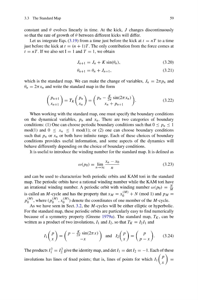
which is the standard map. We can make the change of variables, J n = 2πp n and
θ n = 2πx n and write the standard map in the form
p n+1
x n+1
= T K
p n
x n
=
p n −
K
2π sin(2πx n )
x n + p n+1
.
(3.22)
When working with the standard map, one must specify the boundary conditions
on the dynamical variables, p n and x n . There are two categories of boundary
conditions: (1) One can choose periodic boundary conditions such that 0 ≤ p n ≤ 1
mod(1) and 0 ≤ x n ≤ 1 mod(1); or (2) one can choose boundary conditions
such that p n or x n or both have infinite range. Each of these choices of boundary
conditions provides useful information, and some aspects of the dynamics will
behave differently depending on the choice of boundary conditions.
It is useful to introduce the winding number for the standard map. It is defined as
ω(p 0 ) = lim
n→∞
x n − x 0
n
(3.23)
and can be used to characterize both periodic orbits and KAM tori in the standard
map. The periodic orbits have a rational winding number while the KAM tori have
an irrational winding number. A periodic orbit with winding number ω(p 0 ) =
N
M
is called an M-cycle and has the property that x M = x
(M)
0
+ N (mod 1) and p M =
p
(M)
0 , where (p
(M)
0 , x
(M)
0 ) denote the coordinates of one member of the M-cycle.
As we have seen in Sect. 3.2, the M-cycles will be either elliptic or hyperbolic.
For the standard map, these periodic orbits are particularly easy to find numerically
because of a symmetry property (Greene 1979a). The standard map, T K , can be
written as a product of two involutions, I 1 and I 2 , so that T K = I 2 I 1 and
I 1
p
x
=
p −
K
2π sin(2πx)
−x
and I 2
p
x
=
p
p − x
.
(3.24)
The products I 2
1 = I 2
2 give the identity map, and det I 1 = det I 2 = −1. Each of these
involutions has lines of fixed points; that is, lines of points for which I 1
p
x
=
59
constant and θ evolves linearly in time. At the kick, J changes discontinuously
so that the rate of growth of θ between different kicks will differ.
Let us integrate Eqs. (3.19) from a time just before the kick at t = nT to a time
just before the kick at t = (n + 1)T . The only contribution from the force comes at
t = nT . If we also set I = 1 and T = 1, we obtain
J n+1 = J n + K sin(θ n ),
(3.20)
θ n+1 = θ n + J n+1 ,
(3.21)
which is the standard map. We can make the change of variables, J n = 2πp n and
θ n = 2πx n and write the standard map in the form
p n+1
x n+1
= T K
p n
x n
=
p n −
K
2π sin(2πx n )
x n + p n+1
.
(3.22)
When working with the standard map, one must specify the boundary conditions
on the dynamical variables, p n and x n . There are two categories of boundary
conditions: (1) One can choose periodic boundary conditions such that 0 ≤ p n ≤ 1
mod(1) and 0 ≤ x n ≤ 1 mod(1); or (2) one can choose boundary conditions
such that p n or x n or both have infinite range. Each of these choices of boundary
conditions provides useful information, and some aspects of the dynamics will
behave differently depending on the choice of boundary conditions.
It is useful to introduce the winding number for the standard map. It is defined as
ω(p 0 ) = lim
n→∞
x n − x 0
n
(3.23)
and can be used to characterize both periodic orbits and KAM tori in the standard
map. The periodic orbits have a rational winding number while the KAM tori have
an irrational winding number. A periodic orbit with winding number ω(p 0 ) =
N
M
is called an M-cycle and has the property that x M = x
(M)
0
+ N (mod 1) and p M =
p
(M)
0 , where (p
(M)
0 , x
(M)
0 ) denote the coordinates of one member of the M-cycle.
As we have seen in Sect. 3.2, the M-cycles will be either elliptic or hyperbolic.
For the standard map, these periodic orbits are particularly easy to find numerically
because of a symmetry property (Greene 1979a). The standard map, T K , can be
written as a product of two involutions, I 1 and I 2 , so that T K = I 2 I 1 and
I 1
p
x
=
p −
K
2π sin(2πx)
−x
and I 2
p
x
=
p
p − x
.
(3.24)
The products I 2
1 = I 2
2 give the identity map, and det I 1 = det I 2 = −1. Each of these
involutions has lines of fixed points; that is, lines of points for which I 1
p
x
=