

38
2 Fundamental Concepts
λ i = −λ 2N −i+1 .
(2.79)
On the energy surface, there are 2N − 1 exponents. One of them is zero (the one
associated with motion along the direction of the flow). We can now order the
exponents in order of increasing value. If we relabel the indices in Eq. (2.79), we
can write
−λ N −1 ≤ . . . ≤ −λ 1 ≤ 0 ≤ λ 1 ≤ . . . ≤ λ N −1 .
If t is chosen arbitrarily, it should contain some contribution from all spatial
directions. Then we will find λ(X N
o , Y N
o ) = λ N −1 . A numerical method for
computing all 2N of the Lyapounov exponents in an N degree of freedom system
can be found in Benettin et al. (1979).
Benettin et al. (1976) have computed λ N −1 for the Henon-Heiles system. For
bounded systems, the quantity defined in Eq. (2.77) can be expected to saturate after
a finite time. Thus a slightly different procedure is used to obtain the exponents. One
essentially computes a sequence of distances each of which is obtained after a finite
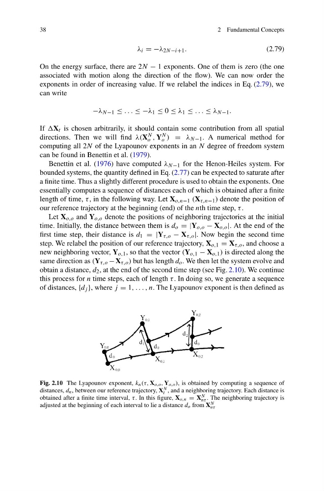
length of time, τ , in the following way. Let X o,n−1 (X τ,n−1 ) denote the position of
our reference trajectory at the beginning (end) of the nth time step, τ .
Let X o,o and Y o,o denote the positions of neighboring trajectories at the initial
time. Initially, the distance between them is d o = |Y o,o − X o,o |. At the end of the
first time step, their distance is d 1 = |Y τ,o − X τ,o |. Now begin the second time
step. We relabel the position of our reference trajectory, X o,1 = X τ,o , and choose a
new neighboring vector, Y o,1 , so that the vector (Y o,1 − X o,1 ) is directed along the
same direction as (Y τ,o − X τ,o ) but has length d o . We then let the system evolve and
obtain a distance, d 2 , at the end of the second time step (see Fig. 2.10). We continue
this process for n time steps, each of length τ . In doing so, we generate a sequence
of distances, {d j }, where j = 1, . . . , n. The Lyapounov exponent is then defined as
Fig. 2.10 The Lyapounov exponent, k n (τ, X o,o , Y o,o ), is obtained by computing a sequence of
distances, d n , between our reference trajectory, X N
t , and a neighboring trajectory. Each distance is
obtained after a finite time interval, τ . In this figure, X o,n = X N
nτ . The neighboring trajectory is
adjusted at the beginning of each interval to lie a distance d o from X N
nτ
2 Fundamental Concepts
λ i = −λ 2N −i+1 .
(2.79)
On the energy surface, there are 2N − 1 exponents. One of them is zero (the one
associated with motion along the direction of the flow). We can now order the
exponents in order of increasing value. If we relabel the indices in Eq. (2.79), we
can write
−λ N −1 ≤ . . . ≤ −λ 1 ≤ 0 ≤ λ 1 ≤ . . . ≤ λ N −1 .
If t is chosen arbitrarily, it should contain some contribution from all spatial
directions. Then we will find λ(X N
o , Y N
o ) = λ N −1 . A numerical method for
computing all 2N of the Lyapounov exponents in an N degree of freedom system
can be found in Benettin et al. (1979).
Benettin et al. (1976) have computed λ N −1 for the Henon-Heiles system. For
bounded systems, the quantity defined in Eq. (2.77) can be expected to saturate after
a finite time. Thus a slightly different procedure is used to obtain the exponents. One
essentially computes a sequence of distances each of which is obtained after a finite
length of time, τ , in the following way. Let X o,n−1 (X τ,n−1 ) denote the position of
our reference trajectory at the beginning (end) of the nth time step, τ .
Let X o,o and Y o,o denote the positions of neighboring trajectories at the initial
time. Initially, the distance between them is d o = |Y o,o − X o,o |. At the end of the
first time step, their distance is d 1 = |Y τ,o − X τ,o |. Now begin the second time
step. We relabel the position of our reference trajectory, X o,1 = X τ,o , and choose a
new neighboring vector, Y o,1 , so that the vector (Y o,1 − X o,1 ) is directed along the
same direction as (Y τ,o − X τ,o ) but has length d o . We then let the system evolve and
obtain a distance, d 2 , at the end of the second time step (see Fig. 2.10). We continue
this process for n time steps, each of length τ . In doing so, we generate a sequence
of distances, {d j }, where j = 1, . . . , n. The Lyapounov exponent is then defined as
Fig. 2.10 The Lyapounov exponent, k n (τ, X o,o , Y o,o ), is obtained by computing a sequence of
distances, d n , between our reference trajectory, X N
t , and a neighboring trajectory. Each distance is
obtained after a finite time interval, τ . In this figure, X o,n = X N
nτ . The neighboring trajectory is
adjusted at the beginning of each interval to lie a distance d o from X N
nτ