

506
G Circular Ensembles
and
π
−π
dθ k ¯
σ N,4 (θ i , θ k )· ¯
σ N,4 (θ k , θ j ) = ¯
σ N,4 (θ i , θ j ).
(G.81)
If we integrate over the quaternion determinant of the N ×N quaternion, ¯
Q
(4)
N , we
obtain the relations
π
−π
dx n+1 . . .
π
−π
dθ N Qdet[ ¯
Q
(4)
N ] = (N − n)! Qdet[ ¯
Q
(4)
n (N)],
(G.82)
where ¯
Q
(4)
n (N) is an n×n quaternion with matrix elements ¯
σ N,4 (θ i , θ j ), and
π
−π
dθ 1 . . .
π
−π
dθ N Qdet[ ¯
Q
(4)
N ] = N!
1 0
0 1
.
(G.83)
We can use the fact that ¯
Q
(4)
N is self-dual to obtain a relation between the
quaternion determinant, Qdet[ ¯
Q
(4)
N ], and the probability density, P N 4 (θ 1 , . . ., θ N ).
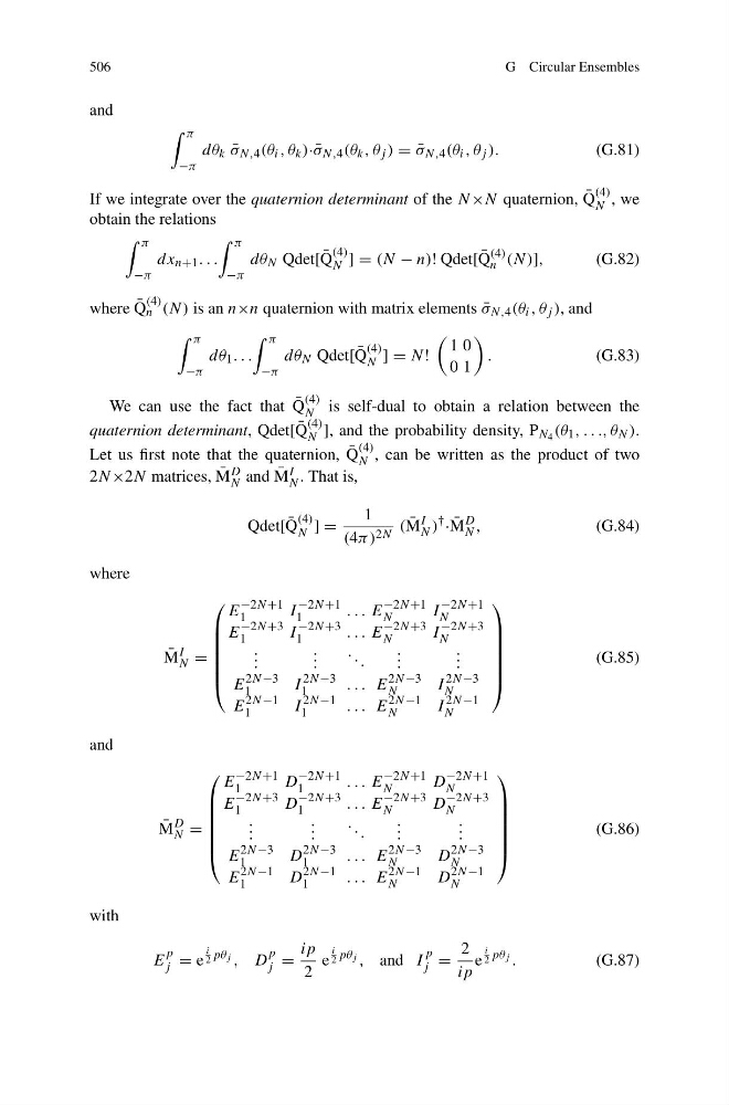
Let us first note that the quaternion, ¯
Q
(4)
N , can be written as the product of two
2N ×2N matrices, ¯
M D
N and ¯
M I
N . That is,
Qdet[ ¯
Q
(4)
N ] =
1
(4π) 2N ( ¯
M
I
N )
†
· ¯
M
D
N ,
(G.84)
where
¯
M
I
N =
⎛
⎜
⎜
⎜
⎜
⎜
⎝
E
−2N +1
1
I
−2N +1
1
. . . E
−2N +1
N
I
−2N +1
N
E
−2N +3
1
I
−2N +3
1
. . . E
−2N +3
N
I
−2N +3
N
. . .
. . .
. . .
. . .
. . .
E
2N −3
1
I
2N −3
1
. . . E
2N −3
N
I
2N −3
N
E
2N −1
1
I
2N −1
1
. . . E
2N −1
N
I
2N −1
N
⎞
⎟
⎟
⎟
⎟
⎟
⎠
(G.85)
and
¯
M
D
N =
⎛
⎜
⎜
⎜
⎜
⎜
⎝
E
−2N +1
1
D
−2N +1
1
. . . E
−2N +1
N
D
−2N +1
N
E
−2N +3
1
D
−2N +3
1
. . . E
−2N +3
N
D
−2N +3
N
. . .
. . .
. . .
. . .
. . .
E
2N −3
1
D
2N −3
1
. . . E
2N −3
N
D
2N −3
N
E
2N −1
1
D
2N −1
1
. . . E
2N −1
N
D
2N −1
N
⎞
⎟
⎟
⎟
⎟
⎟
⎠
(G.86)
with
E
p
j = e
i
2 pθ j , D
p
j =
ip
2
e
i
2 pθ j , and I
p
j =
2
ip
e
i
2 pθ j .
(G.87)
G Circular Ensembles
and
π
−π
dθ k ¯
σ N,4 (θ i , θ k )· ¯
σ N,4 (θ k , θ j ) = ¯
σ N,4 (θ i , θ j ).
(G.81)
If we integrate over the quaternion determinant of the N ×N quaternion, ¯
Q
(4)
N , we
obtain the relations
π
−π
dx n+1 . . .
π
−π
dθ N Qdet[ ¯
Q
(4)
N ] = (N − n)! Qdet[ ¯
Q
(4)
n (N)],
(G.82)
where ¯
Q
(4)
n (N) is an n×n quaternion with matrix elements ¯
σ N,4 (θ i , θ j ), and
π
−π
dθ 1 . . .
π
−π
dθ N Qdet[ ¯
Q
(4)
N ] = N!
1 0
0 1
.
(G.83)
We can use the fact that ¯
Q
(4)
N is self-dual to obtain a relation between the
quaternion determinant, Qdet[ ¯
Q
(4)
N ], and the probability density, P N 4 (θ 1 , . . ., θ N ).
Let us first note that the quaternion, ¯
Q
(4)
N , can be written as the product of two
2N ×2N matrices, ¯
M D
N and ¯
M I
N . That is,
Qdet[ ¯
Q
(4)
N ] =
1
(4π) 2N ( ¯
M
I
N )
†
· ¯
M
D
N ,
(G.84)
where
¯
M
I
N =
⎛
⎜
⎜
⎜
⎜
⎜
⎝
E
−2N +1
1
I
−2N +1
1
. . . E
−2N +1
N
I
−2N +1
N
E
−2N +3
1
I
−2N +3
1
. . . E
−2N +3
N
I
−2N +3
N
. . .
. . .
. . .
. . .
. . .
E
2N −3
1
I
2N −3
1
. . . E
2N −3
N
I
2N −3
N
E
2N −1
1
I
2N −1
1
. . . E
2N −1
N
I
2N −1
N
⎞
⎟
⎟
⎟
⎟
⎟
⎠
(G.85)
and
¯
M
D
N =
⎛
⎜
⎜
⎜
⎜
⎜
⎝
E
−2N +1
1
D
−2N +1
1
. . . E
−2N +1
N
D
−2N +1
N
E
−2N +3
1
D
−2N +3
1
. . . E
−2N +3
N
D
−2N +3
N
. . .
. . .
. . .
. . .
. . .
E
2N −3
1
D
2N −3
1
. . . E
2N −3
N
D
2N −3
N
E
2N −1
1
D
2N −1
1
. . . E
2N −1
N
D
2N −1
N
⎞
⎟
⎟
⎟
⎟
⎟
⎠
(G.86)
with
E
p
j = e
i
2 pθ j , D
p
j =
ip
2
e
i
2 pθ j , and I
p
j =
2
ip
e
i
2 pθ j .
(G.87)