

498
G Circular Ensembles
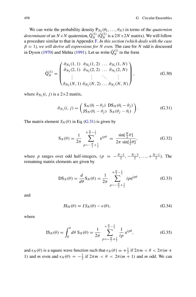
We can write the probability density P N 1 (θ 1 , . . ., θ N ) in terms of the quaternion
determinant of an N×N quaternion, ¯
Q
(1)
N ( ¯
Q
(1)
N is a 2N ×2N matrix). We will follow
a procedure similar to that in Appendix F. In this section (which deals with the case
β = 1), we will derive all expressions for N even. The case for N odd is discussed
in Dyson (1970) and Mehta (1991). Let us write ¯
Q
(1)
N in the form
¯
Q
(1)
N =
⎛
⎜
⎜
⎜
⎝
¯
σ N 1 (1, 1) ¯
σ N 1 (1, 2) . . . ¯
σ N 1 (1, N)
¯
σ N 1 (2, 1) ¯
σ N 1 (2, 2) . . . ¯
σ N 1 (2, N)
. . .
. . .
. . .
. . .
¯
σ N 1 (N, 1) ¯
σ N 1 (N, 2) . . . ¯
σ N 1 (N, N)
⎞
⎟
⎟
⎟
⎠
,
(G.30)
where ¯
σ N 1 (i, j ) is a 2×2 matrix,
¯
σ N 1 (i, j ) =
S N (θ i − θ j ) DS N (θ i − θ j )
JS N (θ i − θ j ) S N (θ j − θ i )
.
(G.31)
The matrix element S N (θ ) in Eq. (G.31) is given by
S N (θ ) =
1
2π
+
N
2 −
1
2
p=−
N
2 +
1
2
e
ipθ
=
sin[
N
2 θ ]
2π sin[
1
2 θ ]
,
(G.32)
where p ranges over odd half-integers, (p = −
N −1
2 , −
N −3
2 , . . ., +
N −1
2 ). The
remaining matrix elements are given by
DS N (θ ) =
d
dθ
S N (θ ) =
1
2π
+
N
2 −
1
2
p=−
N
2 +
1
2
ipe
ipθ
(G.33)
and
JS N (θ ) = I S N (θ ) − (θ),
(G.34)
where
IS N (θ ) =
θ
0
dθ S N (θ ) =
1
2π
+
N
2 −
1
2
p=−
N
2 +
1
2
1
ip
e
ipθ ,
(G.35)
and N (θ ) is a square wave function such that N (θ ) = +
1
2 if 2πm < θ < 2π(m +
1) and m even and N (θ ) = −
1
2 if 2πm < θ < 2π(m + 1) and m odd. We can
G Circular Ensembles
We can write the probability density P N 1 (θ 1 , . . ., θ N ) in terms of the quaternion
determinant of an N×N quaternion, ¯
Q
(1)
N ( ¯
Q
(1)
N is a 2N ×2N matrix). We will follow
a procedure similar to that in Appendix F. In this section (which deals with the case
β = 1), we will derive all expressions for N even. The case for N odd is discussed
in Dyson (1970) and Mehta (1991). Let us write ¯
Q
(1)
N in the form
¯
Q
(1)
N =
⎛
⎜
⎜
⎜
⎝
¯
σ N 1 (1, 1) ¯
σ N 1 (1, 2) . . . ¯
σ N 1 (1, N)
¯
σ N 1 (2, 1) ¯
σ N 1 (2, 2) . . . ¯
σ N 1 (2, N)
. . .
. . .
. . .
. . .
¯
σ N 1 (N, 1) ¯
σ N 1 (N, 2) . . . ¯
σ N 1 (N, N)
⎞
⎟
⎟
⎟
⎠
,
(G.30)
where ¯
σ N 1 (i, j ) is a 2×2 matrix,
¯
σ N 1 (i, j ) =
S N (θ i − θ j ) DS N (θ i − θ j )
JS N (θ i − θ j ) S N (θ j − θ i )
.
(G.31)
The matrix element S N (θ ) in Eq. (G.31) is given by
S N (θ ) =
1
2π
+
N
2 −
1
2
p=−
N
2 +
1
2
e
ipθ
=
sin[
N
2 θ ]
2π sin[
1
2 θ ]
,
(G.32)
where p ranges over odd half-integers, (p = −
N −1
2 , −
N −3
2 , . . ., +
N −1
2 ). The
remaining matrix elements are given by
DS N (θ ) =
d
dθ
S N (θ ) =
1
2π
+
N
2 −
1
2
p=−
N
2 +
1
2
ipe
ipθ
(G.33)
and
JS N (θ ) = I S N (θ ) − (θ),
(G.34)
where
IS N (θ ) =
θ
0
dθ S N (θ ) =
1
2π
+
N
2 −
1
2
p=−
N
2 +
1
2
1
ip
e
ipθ ,
(G.35)
and N (θ ) is a square wave function such that N (θ ) = +
1
2 if 2πm < θ < 2π(m +
1) and m even and N (θ ) = −
1
2 if 2πm < θ < 2π(m + 1) and m odd. We can