

478
F Gaussian Ensembles
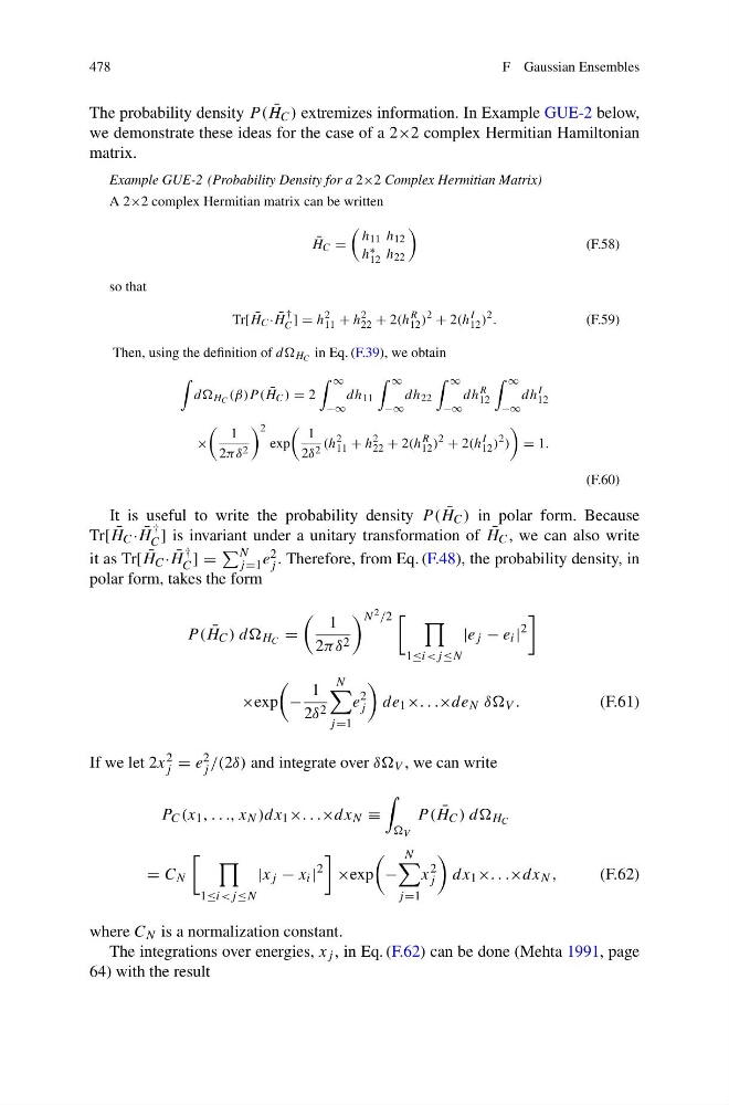
The probability density P ( ¯
H C ) extremizes information. In Example GUE-2 below,
we demonstrate these ideas for the case of a 2×2 complex Hermitian Hamiltonian
matrix.
Example GUE-2 (Probability Density for a 2×2 Complex Hermitian Matrix)
A 2×2 complex Hermitian matrix can be written
¯
H C =
h 11 h 12
h ∗
12 h 22
(F.58)
so that
Tr[ ¯
H C · ¯
H
†
C ] = h
2
11 + h
2
22 + 2(h
R
12 )
2 + 2(h
I
12 )
2 .
(F.59)
Then, using the definition of dd H C in Eq. (F.39), we obtain
dd H C (β)P ( ¯
H C ) = 2
∞
−∞
dh 11
∞
−∞
dh 22
∞
−∞
dh
R
12
∞
−∞
dh
I
12
×
1
2πδ 2
2
exp
1
2δ 2 (h
2
11 + h
2
22 + 2(h
R
12 )
2 + 2(h
I
12 )
2 )
= 1.
(F.60)
It is useful to write the probability density P ( ¯
H C ) in polar form. Because
Tr[ ¯
H C · ¯
H
†
C ] is invariant under a unitary transformation of ¯
H C , we can also write
it as Tr[ ¯
H C · ¯
H
†
C ] =
N
j =1 e 2
j . Therefore, from Eq. (F.48), the probability density, in
polar form, takes the form
P ( ¯
H C ) dd H C =
1
2πδ 2
N 2 /2
1≤i
2
×exp
−
1
2δ 2
N
j =1
e
2
j
de 1 ×. . .×de N δδ V .
(F.61)
If we let 2x 2
j = e 2
j /(2δ) and integrate over δδ V , we can write
P C (x 1 , . . ., x N )dx 1 ×. . .×dx N ≡
V
P ( ¯
H C ) dd H C
= C N
1≤i
2
×exp
−
N
j =1
x
2
j
dx 1 ×. . .×dx N ,
(F.62)
where C N is a normalization constant.
The integrations over energies, x j , in Eq. (F.62) can be done (Mehta 1991, page
64) with the result
F Gaussian Ensembles
The probability density P ( ¯
H C ) extremizes information. In Example GUE-2 below,
we demonstrate these ideas for the case of a 2×2 complex Hermitian Hamiltonian
matrix.
Example GUE-2 (Probability Density for a 2×2 Complex Hermitian Matrix)
A 2×2 complex Hermitian matrix can be written
¯
H C =
h 11 h 12
h ∗
12 h 22
(F.58)
so that
Tr[ ¯
H C · ¯
H
†
C ] = h
2
11 + h
2
22 + 2(h
R
12 )
2 + 2(h
I
12 )
2 .
(F.59)
Then, using the definition of dd H C in Eq. (F.39), we obtain
dd H C (β)P ( ¯
H C ) = 2
∞
−∞
dh 11
∞
−∞
dh 22
∞
−∞
dh
R
12
∞
−∞
dh
I
12
×
1
2πδ 2
2
exp
1
2δ 2 (h
2
11 + h
2
22 + 2(h
R
12 )
2 + 2(h
I
12 )
2 )
= 1.
(F.60)
It is useful to write the probability density P ( ¯
H C ) in polar form. Because
Tr[ ¯
H C · ¯
H
†
C ] is invariant under a unitary transformation of ¯
H C , we can also write
it as Tr[ ¯
H C · ¯
H
†
C ] =
N
j =1 e 2
j . Therefore, from Eq. (F.48), the probability density, in
polar form, takes the form
P ( ¯
H C ) dd H C =
1
2πδ 2
N 2 /2
1≤i
2
×exp
−
1
2δ 2
N
j =1
e
2
j
de 1 ×. . .×de N δδ V .
(F.61)
If we let 2x 2
j = e 2
j /(2δ) and integrate over δδ V , we can write
P C (x 1 , . . ., x N )dx 1 ×. . .×dx N ≡
V
P ( ¯
H C ) dd H C
= C N
1≤i
2
×exp
−
N
j =1
x
2
j
dx 1 ×. . .×dx N ,
(F.62)
where C N is a normalization constant.
The integrations over energies, x j , in Eq. (F.62) can be done (Mehta 1991, page
64) with the result