

F.2 Gaussian Unitary Ensemble (GUE)
477
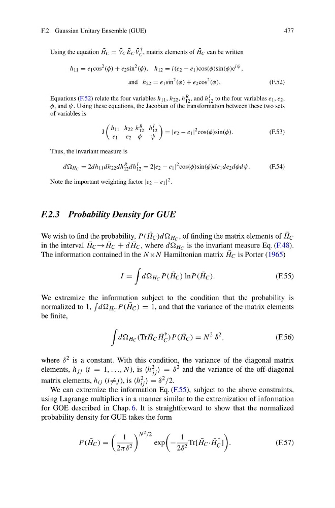
Using the equation ¯
H C = ¯
V C ¯
E C ¯
V
†
C , matrix elements of ¯
H C can be written
h 11 = e 1 cos
2 (φ) + e 2 sin
2 (φ), h 12 = i(e 2 − e 1 )cos(φ)sin(φ)e
iψ ,
and h 22 = e 1 sin
2 (φ) + e 2 cos
2 (φ).
(F.52)
Equations (F.52) relate the four variables h 11 , h 22 , h R
12 , and h I
12 to the four variables e 1 , e 2 ,
φ, and ψ. Using these equations, the Jacobian of the transformation between these two sets
of variables is
J
h 11 h 22 h R
12 h I
12
e 1 e 2 φ ψ
= |e 2 − e 1 |
2 cos(φ)sin(φ).
(F.53)
Thus, the invariant measure is
dd H C = 2dh 11 dh 22 dh
R
12 dh
I
12 = 2|e 2 − e 1 |
2 cos(φ)sin(φ)de 1 de 2 dφdψ.
(F.54)
Note the important weighting factor |e 2 − e 1 | 2 .
F.2.3 Probability Density for GUE
We wish to find the probability, P ( ¯
H C )dd H C , of finding the matrix elements of ¯
H C
in the interval ¯
H C → ¯
H C + d ¯
H C , where dd H C is the invariant measure Eq. (F.48).
The information contained in the N×N Hamiltonian matrix ¯
H C is Porter (1965)
I =
dd H C P ( ¯
H C ) lnP ( ¯
H C ).
(F.55)
We extremize the information subject to the condition that the probability is
normalized to 1,
dd H C P ( ¯
H C ) = 1, and that the variance of the matrix elements
be finite,
dd H C (Tr ¯
H C ¯
H
†
C )P ( ¯
H C ) = N
2 δ
2 ,
(F.56)
where δ 2 is a constant. With this condition, the variance of the diagonal matrix
elements, h jj (i = 1, . . ., N), is h 2
jj = δ 2 and the variance of the off-diagonal
matrix elements, h ij (i =j ), is h 2
ij = δ 2 /2.
We can extremize the information Eq. (F.55), subject to the above constraints,
using Lagrange multipliers in a manner similar to the extremization of information
for GOE described in Chap. 6. It is straightforward to show that the normalized
probability density for GUE takes the form
P ( ¯
H C ) =
1
2πδ 2
N 2 /2
exp
−
1
2δ 2 Tr[ ¯
H C · ¯
H
†
C ]
.
(F.57)
477
Using the equation ¯
H C = ¯
V C ¯
E C ¯
V
†
C , matrix elements of ¯
H C can be written
h 11 = e 1 cos
2 (φ) + e 2 sin
2 (φ), h 12 = i(e 2 − e 1 )cos(φ)sin(φ)e
iψ ,
and h 22 = e 1 sin
2 (φ) + e 2 cos
2 (φ).
(F.52)
Equations (F.52) relate the four variables h 11 , h 22 , h R
12 , and h I
12 to the four variables e 1 , e 2 ,
φ, and ψ. Using these equations, the Jacobian of the transformation between these two sets
of variables is
J
h 11 h 22 h R
12 h I
12
e 1 e 2 φ ψ
= |e 2 − e 1 |
2 cos(φ)sin(φ).
(F.53)
Thus, the invariant measure is
dd H C = 2dh 11 dh 22 dh
R
12 dh
I
12 = 2|e 2 − e 1 |
2 cos(φ)sin(φ)de 1 de 2 dφdψ.
(F.54)
Note the important weighting factor |e 2 − e 1 | 2 .
F.2.3 Probability Density for GUE
We wish to find the probability, P ( ¯
H C )dd H C , of finding the matrix elements of ¯
H C
in the interval ¯
H C → ¯
H C + d ¯
H C , where dd H C is the invariant measure Eq. (F.48).
The information contained in the N×N Hamiltonian matrix ¯
H C is Porter (1965)
I =
dd H C P ( ¯
H C ) lnP ( ¯
H C ).
(F.55)
We extremize the information subject to the condition that the probability is
normalized to 1,
dd H C P ( ¯
H C ) = 1, and that the variance of the matrix elements
be finite,
dd H C (Tr ¯
H C ¯
H
†
C )P ( ¯
H C ) = N
2 δ
2 ,
(F.56)
where δ 2 is a constant. With this condition, the variance of the diagonal matrix
elements, h jj (i = 1, . . ., N), is h 2
jj = δ 2 and the variance of the off-diagonal
matrix elements, h ij (i =j ), is h 2
ij = δ 2 /2.
We can extremize the information Eq. (F.55), subject to the above constraints,
using Lagrange multipliers in a manner similar to the extremization of information
for GOE described in Chap. 6. It is straightforward to show that the normalized
probability density for GUE takes the form
P ( ¯
H C ) =
1
2πδ 2
N 2 /2
exp
−
1
2δ 2 Tr[ ¯
H C · ¯
H
†
C ]
.
(F.57)