

2.6 KAM Theory
33
mogorov’s ideas were made rigorous by Arnol’d (1963) and by Moser (1962). The
nonresonant tori that have not been destroyed by resonances are called KAM tori or
KAM surfaces (after Kolmogorov, Arnol’d, and Moser). Examples of KAM tori can
be found in Figs. 2.7 and 2.8, and many more will be seen throughout this book.
The KAM theory applies to systems with N degrees of freedom whose motion is
governed by a Hamiltonian of the form
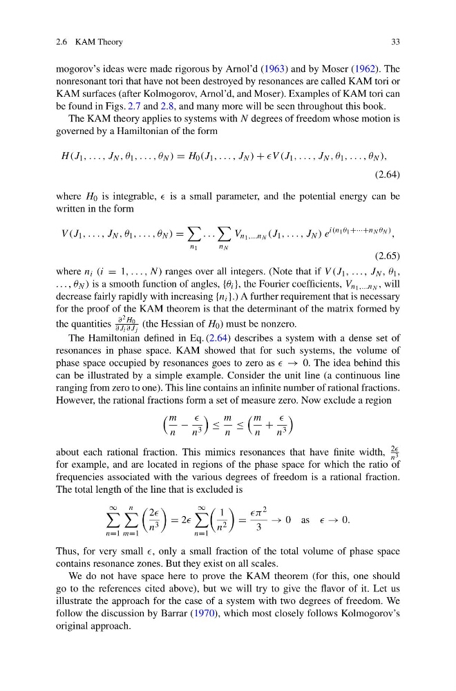
H (J 1 , . . . , J N , θ 1 , . . . , θ N ) = H 0 (J 1 , . . . , J N ) + V (J 1 , . . . , J N , θ 1 , . . . , θ N ),
(2.64)
where H 0 is integrable, is a small parameter, and the potential energy can be
written in the form
V (J 1 , . . . , J N , θ 1 , . . . , θ N ) =
n 1
. . .
n N
V n 1 ,...n N (J 1 , . . . , J N ) e
i(n 1 θ 1 +···+n N θ N ) ,
(2.65)
where n i (i = 1, . . . , N) ranges over all integers. (Note that if V (J 1 , . . . , J N , θ 1 ,
. . . , θ N ) is a smooth function of angles, {θ i }, the Fourier coefficients, V n 1 ,...n N , will
decrease fairly rapidly with increasing {n i }.) A further requirement that is necessary
for the proof of the KAM theorem is that the determinant of the matrix formed by
the quantities
∂ 2 H 0
∂J i ∂J j
(the Hessian of H 0 ) must be nonzero.
The Hamiltonian defined in Eq. (2.64) describes a system with a dense set of
resonances in phase space. KAM showed that for such systems, the volume of
phase space occupied by resonances goes to zero as → 0. The idea behind this
can be illustrated by a simple example. Consider the unit line (a continuous line
ranging from zero to one). This line contains an infinite number of rational fractions.
However, the rational fractions form a set of measure zero. Now exclude a region
m
n
−
n 3
≤
m
n
≤
m
n
+
n 3
about each rational fraction. This mimics resonances that have finite width,
2
n 3
for example, and are located in regions of the phase space for which the ratio of
frequencies associated with the various degrees of freedom is a rational fraction.
The total length of the line that is excluded is
∞
n=1
n
m=1
2
n 3
= 2
∞
n=1
1
n 2
=
π 2
3
→ 0 as → 0.
Thus, for very small , only a small fraction of the total volume of phase space
contains resonance zones. But they exist on all scales.
We do not have space here to prove the KAM theorem (for this, one should
go to the references cited above), but we will try to give the flavor of it. Let us
illustrate the approach for the case of a system with two degrees of freedom. We
follow the discussion by Barrar (1970), which most closely follows Kolmogorov’s
original approach.
33
mogorov’s ideas were made rigorous by Arnol’d (1963) and by Moser (1962). The
nonresonant tori that have not been destroyed by resonances are called KAM tori or
KAM surfaces (after Kolmogorov, Arnol’d, and Moser). Examples of KAM tori can
be found in Figs. 2.7 and 2.8, and many more will be seen throughout this book.
The KAM theory applies to systems with N degrees of freedom whose motion is
governed by a Hamiltonian of the form
H (J 1 , . . . , J N , θ 1 , . . . , θ N ) = H 0 (J 1 , . . . , J N ) + V (J 1 , . . . , J N , θ 1 , . . . , θ N ),
(2.64)
where H 0 is integrable, is a small parameter, and the potential energy can be
written in the form
V (J 1 , . . . , J N , θ 1 , . . . , θ N ) =
n 1
. . .
n N
V n 1 ,...n N (J 1 , . . . , J N ) e
i(n 1 θ 1 +···+n N θ N ) ,
(2.65)
where n i (i = 1, . . . , N) ranges over all integers. (Note that if V (J 1 , . . . , J N , θ 1 ,
. . . , θ N ) is a smooth function of angles, {θ i }, the Fourier coefficients, V n 1 ,...n N , will
decrease fairly rapidly with increasing {n i }.) A further requirement that is necessary
for the proof of the KAM theorem is that the determinant of the matrix formed by
the quantities
∂ 2 H 0
∂J i ∂J j
(the Hessian of H 0 ) must be nonzero.
The Hamiltonian defined in Eq. (2.64) describes a system with a dense set of
resonances in phase space. KAM showed that for such systems, the volume of
phase space occupied by resonances goes to zero as → 0. The idea behind this
can be illustrated by a simple example. Consider the unit line (a continuous line
ranging from zero to one). This line contains an infinite number of rational fractions.
However, the rational fractions form a set of measure zero. Now exclude a region
m
n
−
n 3
≤
m
n
≤
m
n
+
n 3
about each rational fraction. This mimics resonances that have finite width,
2
n 3
for example, and are located in regions of the phase space for which the ratio of
frequencies associated with the various degrees of freedom is a rational fraction.
The total length of the line that is excluded is
∞
n=1
n
m=1
2
n 3
= 2
∞
n=1
1
n 2
=
π 2
3
→ 0 as → 0.
Thus, for very small , only a small fraction of the total volume of phase space
contains resonance zones. But they exist on all scales.
We do not have space here to prove the KAM theorem (for this, one should
go to the references cited above), but we will try to give the flavor of it. Let us
illustrate the approach for the case of a system with two degrees of freedom. We
follow the discussion by Barrar (1970), which most closely follows Kolmogorov’s
original approach.