

Appendix E
Quaternions
The mathematical properties of quaternions play an important role in the random
matrix theory of quantum systems. In subsequent sections, we first define and
describe some general properties of quaternions. We use quaternions to derive some
important properties of matrices that appear in the Gaussian Orthogonal Ensemble.
E.1 General Properties of Quaternions
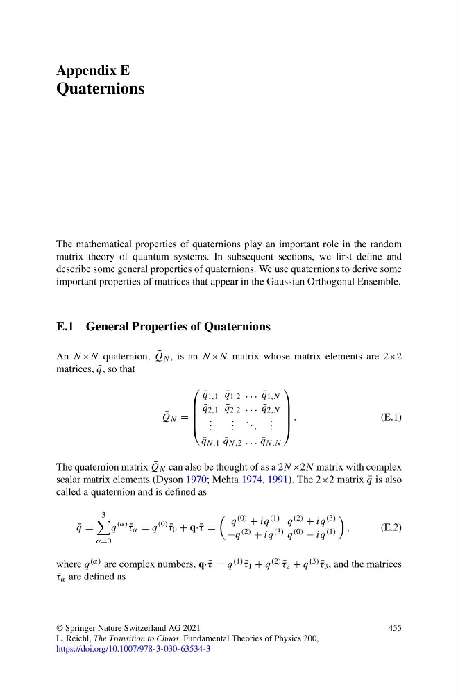
An N ×N quaternion, ¯
Q N , is an N×N matrix whose matrix elements are 2×2
matrices, ¯
q, so that
¯
Q N =
⎛
⎜
⎜
⎜
⎝
¯
q 1,1 ¯
q 1,2 . . . ¯
q 1,N
¯
q 2,1 ¯
q 2,2 . . . ¯
q 2,N
. . .
. . .
. . .
. . .
¯
q N,1 ¯
q N,2 . . . ¯
q N,N
⎞
⎟
⎟
⎟
⎠
.
(E.1)
The quaternion matrix ¯
Q N can also be thought of as a 2N ×2N matrix with complex
scalar matrix elements (Dyson 1970; Mehta 1974, 1991). The 2×2 matrix ¯
q is also
called a quaternion and is defined as
¯
q =
3
α=0
q
(α)
¯
τ α = q
(0)
¯
τ 0 + q· ¯
τ =
q (0) + iq (1) q (2) + iq (3)
−q (2) + iq (3) q (0) − iq (1)
,
(E.2)
where q (α) are complex numbers, q· ¯
τ = q (1) ¯
τ 1 + q (2) ¯
τ 2 + q (3) ¯
τ 3 , and the matrices
¯
τ α are defined as
© Springer Nature Switzerland AG 2021
L. Reichl, The Transition to Chaos, Fundamental Theories of Physics 200,
https://doi.org/10.1007/978-3-030-63534-3
455
Quaternions
The mathematical properties of quaternions play an important role in the random
matrix theory of quantum systems. In subsequent sections, we first define and
describe some general properties of quaternions. We use quaternions to derive some
important properties of matrices that appear in the Gaussian Orthogonal Ensemble.
E.1 General Properties of Quaternions
An N ×N quaternion, ¯
Q N , is an N×N matrix whose matrix elements are 2×2
matrices, ¯
q, so that
¯
Q N =
⎛
⎜
⎜
⎜
⎝
¯
q 1,1 ¯
q 1,2 . . . ¯
q 1,N
¯
q 2,1 ¯
q 2,2 . . . ¯
q 2,N
. . .
. . .
. . .
. . .
¯
q N,1 ¯
q N,2 . . . ¯
q N,N
⎞
⎟
⎟
⎟
⎠
.
(E.1)
The quaternion matrix ¯
Q N can also be thought of as a 2N ×2N matrix with complex
scalar matrix elements (Dyson 1970; Mehta 1974, 1991). The 2×2 matrix ¯
q is also
called a quaternion and is defined as
¯
q =
3
α=0
q
(α)
¯
τ α = q
(0)
¯
τ 0 + q· ¯
τ =
q (0) + iq (1) q (2) + iq (3)
−q (2) + iq (3) q (0) − iq (1)
,
(E.2)
where q (α) are complex numbers, q· ¯
τ = q (1) ¯
τ 1 + q (2) ¯
τ 2 + q (3) ¯
τ 3 , and the matrices
¯
τ α are defined as
© Springer Nature Switzerland AG 2021
L. Reichl, The Transition to Chaos, Fundamental Theories of Physics 200,
https://doi.org/10.1007/978-3-030-63534-3
455