

D.3 Unitary Matrices
441
D.3 Unitary Matrices
Unitary matrices are especially important for scattering theory since most scattering
properties are determined by the unitary S-matrix (scattering matrix), which connects incoming states to outgoing states in the scattering process. Unitary matrices,
called Floquet matrices, are also widely used to describe the time evolution of
quantum systems that are driven by time-periodic external forces.
An N×N unitary matrix, ¯
U , is a complex square matrix that is constrained by
the condition
¯
U
†
= ¯
U
−1 so ¯
U
†
· ¯
U = ¯
U · ¯
U
†
= ¯
I ,
(D.50)
where ¯
I is an N ×N unit matrix. It is useful to introduce the parametric representation of the unitary matrix,
¯
U =
( ¯
I + i ¯
H )
( ¯
I − i ¯
H )
,
(D.51)
where ¯
H is a Hermitian matrix. The Hermitian matrix, ¯
H , can be diagonalized by a
unitary matrix, ¯
V , so that
¯
H = ¯
V ¯
E ¯
V
† .
(D.52)
If ¯
H = ¯
H R is a real symmetric matrix, then ¯
E = ¯
E R (see Eq. (D.11)) and ¯
V is
complex and symmetric. If ¯
H = ¯
H C is a complex Hermitian matrix, then ¯
E = ¯
E C
(see Eq. (D.24)) and ¯
V is unitary. If ¯
H = ¯
H Q is a quaternion real matrix, then ¯
E =
¯
E Q (see Eq. (D.42 )) and ¯
V is a symplectic unitary matrix. Because of Eq. (D.51),
the unitary matrix, ¯
U will also be diagonalized by the unitary matrix, ¯
V , so that
¯
U = ¯
V ¯
¯
V
† ,
(D.53)
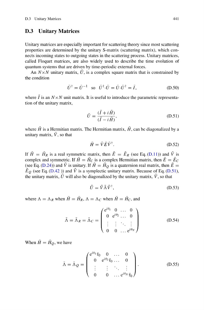
where = R when ¯
H = ¯
H R , = C when ¯
H = ¯
H C , and
¯
= ¯
R = ¯
C =
⎛
⎜
⎜
⎜
⎝
e iθ 1 0 . . . 0
0 e iθ 2 . . . 0
. . .
. . .
. . .
. . .
0 0 . . . e iθ N
⎞
⎟
⎟
⎟
⎠
(D.54)
When ¯
H = ¯
H Q , we have
¯
= ¯
Q =
⎛
⎜
⎜
⎜
⎝
e iθ 1 ¯
τ 0 0 . . . 0
0 e iθ 2 ¯
τ 0 . . . 0
. . .
. . .
. . .
. . .
0
0 . . . e iθ N ¯
τ 0
⎞
⎟
⎟
⎟
⎠
.
(D.55)
441
D.3 Unitary Matrices
Unitary matrices are especially important for scattering theory since most scattering
properties are determined by the unitary S-matrix (scattering matrix), which connects incoming states to outgoing states in the scattering process. Unitary matrices,
called Floquet matrices, are also widely used to describe the time evolution of
quantum systems that are driven by time-periodic external forces.
An N×N unitary matrix, ¯
U , is a complex square matrix that is constrained by
the condition
¯
U
†
= ¯
U
−1 so ¯
U
†
· ¯
U = ¯
U · ¯
U
†
= ¯
I ,
(D.50)
where ¯
I is an N ×N unit matrix. It is useful to introduce the parametric representation of the unitary matrix,
¯
U =
( ¯
I + i ¯
H )
( ¯
I − i ¯
H )
,
(D.51)
where ¯
H is a Hermitian matrix. The Hermitian matrix, ¯
H , can be diagonalized by a
unitary matrix, ¯
V , so that
¯
H = ¯
V ¯
E ¯
V
† .
(D.52)
If ¯
H = ¯
H R is a real symmetric matrix, then ¯
E = ¯
E R (see Eq. (D.11)) and ¯
V is
complex and symmetric. If ¯
H = ¯
H C is a complex Hermitian matrix, then ¯
E = ¯
E C
(see Eq. (D.24)) and ¯
V is unitary. If ¯
H = ¯
H Q is a quaternion real matrix, then ¯
E =
¯
E Q (see Eq. (D.42 )) and ¯
V is a symplectic unitary matrix. Because of Eq. (D.51),
the unitary matrix, ¯
U will also be diagonalized by the unitary matrix, ¯
V , so that
¯
U = ¯
V ¯
¯
V
† ,
(D.53)
where = R when ¯
H = ¯
H R , = C when ¯
H = ¯
H C , and
¯
= ¯
R = ¯
C =
⎛
⎜
⎜
⎜
⎝
e iθ 1 0 . . . 0
0 e iθ 2 . . . 0
. . .
. . .
. . .
. . .
0 0 . . . e iθ N
⎞
⎟
⎟
⎟
⎠
(D.54)
When ¯
H = ¯
H Q , we have
¯
= ¯
Q =
⎛
⎜
⎜
⎜
⎝
e iθ 1 ¯
τ 0 0 . . . 0
0 e iθ 2 ¯
τ 0 . . . 0
. . .
. . .
. . .
. . .
0
0 . . . e iθ N ¯
τ 0
⎞
⎟
⎟
⎟
⎠
.
(D.55)