

2.5 Nonlinear Resonance and Chaos
31
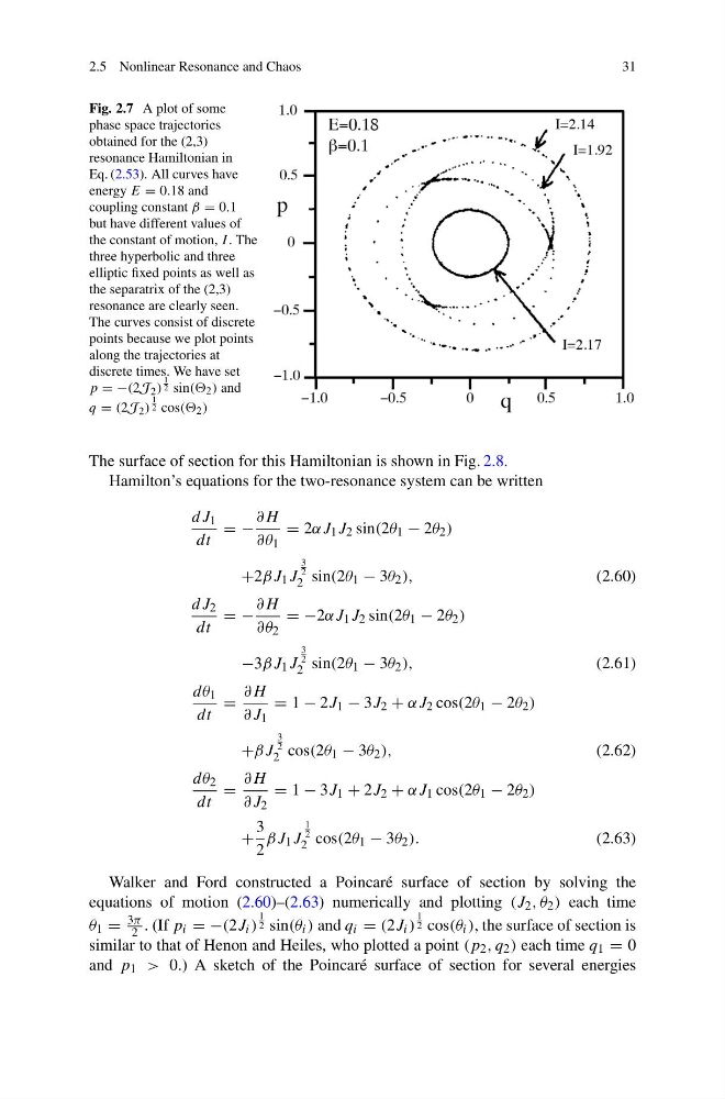
Fig. 2.7 A plot of some
phase space trajectories
obtained for the (2,3)
resonance Hamiltonian in
Eq. (2.53). All curves have
energy E = 0.18 and
coupling constant β = 0.1
but have different values of
the constant of motion, I . The
three hyperbolic and three
elliptic fixed points as well as
the separatrix of the (2,3)
resonance are clearly seen.
The curves consist of discrete
points because we plot points
along the trajectories at
discrete times. We have set
p = −(2J 2 )
1
2 sin(( 2 ) and
q = (2J 2 )
1
2 cos(( 2 )
The surface of section for this Hamiltonian is shown in Fig. 2.8.
Hamilton’s equations for the two-resonance system can be written
dJ 1
dt
= −
∂H
∂θ 1
= 2αJ 1 J 2 sin(2θ 1 − 2θ 2 )
+2βJ 1 J
3
2
2 sin(2θ 1 − 3θ 2 ),
(2.60)
dJ 2
dt
= −
∂H
∂θ 2
= −2αJ 1 J 2 sin(2θ 1 − 2θ 2 )
−3βJ 1 J
3
2
2 sin(2θ 1 − 3θ 2 ),
(2.61)
dθ 1
dt
=
∂H
∂J 1
= 1 − 2J 1 − 3J 2 + αJ 2 cos(2θ 1 − 2θ 2 )
+βJ
3
2
2 cos(2θ 1 − 3θ 2 ),
(2.62)
dθ 2
dt
=
∂H
∂J 2
= 1 − 3J 1 + 2J 2 + αJ 1 cos(2θ 1 − 2θ 2 )
+
3
2
βJ 1 J
1
2
2 cos(2θ 1 − 3θ 2 ).
(2.63)
Walker and Ford constructed a Poincaré surface of section by solving the
equations of motion (2.60)–(2.63) numerically and plotting (J 2 , θ 2 ) each time
θ 1 =
3π
2 . (If p i = −(2J i )
1
2 sin(θ i ) and q i = (2J i )
1
2 cos(θ i ), the surface of section is
similar to that of Henon and Heiles, who plotted a point (p 2 , q 2 ) each time q 1 = 0
and p 1 > 0.) A sketch of the Poincaré surface of section for several energies
31
Fig. 2.7 A plot of some
phase space trajectories
obtained for the (2,3)
resonance Hamiltonian in
Eq. (2.53). All curves have
energy E = 0.18 and
coupling constant β = 0.1
but have different values of
the constant of motion, I . The
three hyperbolic and three
elliptic fixed points as well as
the separatrix of the (2,3)
resonance are clearly seen.
The curves consist of discrete
points because we plot points
along the trajectories at
discrete times. We have set
p = −(2J 2 )
1
2 sin(( 2 ) and
q = (2J 2 )
1
2 cos(( 2 )
The surface of section for this Hamiltonian is shown in Fig. 2.8.
Hamilton’s equations for the two-resonance system can be written
dJ 1
dt
= −
∂H
∂θ 1
= 2αJ 1 J 2 sin(2θ 1 − 2θ 2 )
+2βJ 1 J
3
2
2 sin(2θ 1 − 3θ 2 ),
(2.60)
dJ 2
dt
= −
∂H
∂θ 2
= −2αJ 1 J 2 sin(2θ 1 − 2θ 2 )
−3βJ 1 J
3
2
2 sin(2θ 1 − 3θ 2 ),
(2.61)
dθ 1
dt
=
∂H
∂J 1
= 1 − 2J 1 − 3J 2 + αJ 2 cos(2θ 1 − 2θ 2 )
+βJ
3
2
2 cos(2θ 1 − 3θ 2 ),
(2.62)
dθ 2
dt
=
∂H
∂J 2
= 1 − 3J 1 + 2J 2 + αJ 1 cos(2θ 1 − 2θ 2 )
+
3
2
βJ 1 J
1
2
2 cos(2θ 1 − 3θ 2 ).
(2.63)
Walker and Ford constructed a Poincaré surface of section by solving the
equations of motion (2.60)–(2.63) numerically and plotting (J 2 , θ 2 ) each time
θ 1 =
3π
2 . (If p i = −(2J i )
1
2 sin(θ i ) and q i = (2J i )
1
2 cos(θ i ), the surface of section is
similar to that of Henon and Heiles, who plotted a point (p 2 , q 2 ) each time q 1 = 0
and p 1 > 0.) A sketch of the Poincaré surface of section for several energies