

B.3 Infinite Square-Well Potential
413
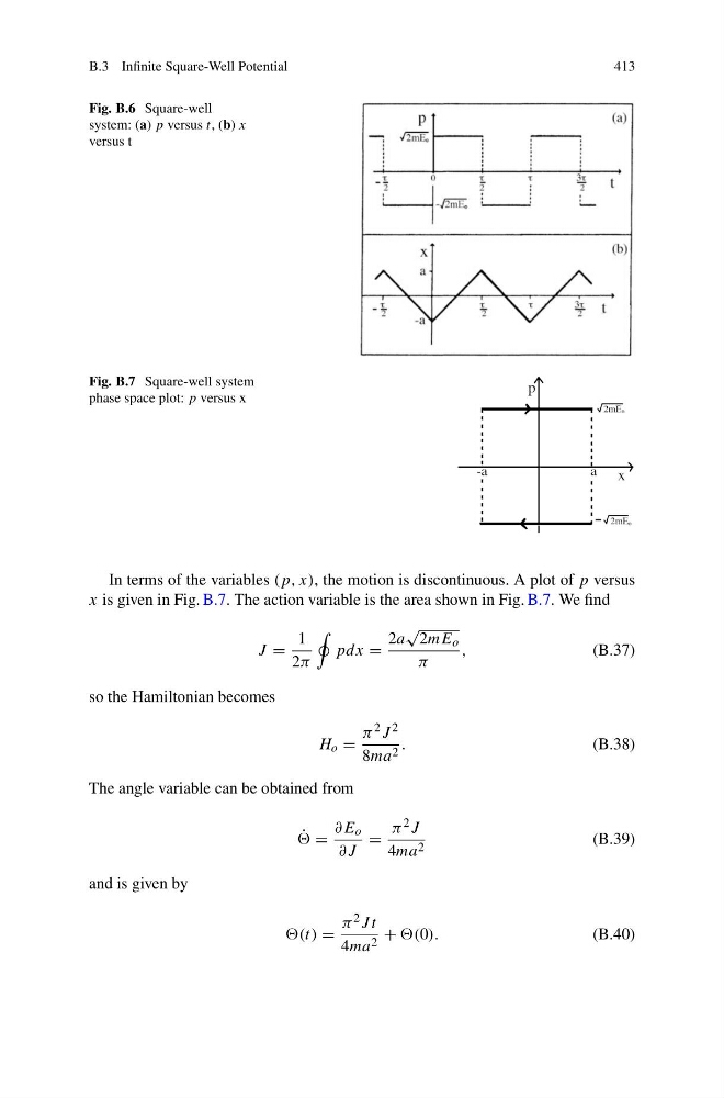
Fig. B.6 Square-well
system: (a) p versus t, (b) x
versus t
Fig. B.7 Square-well system
phase space plot: p versus x
In terms of the variables (p, x), the motion is discontinuous. A plot of p versus
x is given in Fig. B.7. The action variable is the area shown in Fig. B.7. We find
J =
1
2π
pdx =
2a
√
2mE o
π
,
(B.37)
so the Hamiltonian becomes
H o =
π 2 J 2
8ma 2 .
(B.38)
The angle variable can be obtained from
˙
=
∂E o
∂J
=
π 2 J
4ma 2
(B.39)
and is given by
=
π 2 J t
4ma 2 +
(B.40)
413
Fig. B.6 Square-well
system: (a) p versus t, (b) x
versus t
Fig. B.7 Square-well system
phase space plot: p versus x
In terms of the variables (p, x), the motion is discontinuous. A plot of p versus
x is given in Fig. B.7. The action variable is the area shown in Fig. B.7. We find
J =
1
2π
pdx =
2a
√
2mE o
π
,
(B.37)
so the Hamiltonian becomes
H o =
π 2 J 2
8ma 2 .
(B.38)
The angle variable can be obtained from
˙
=
∂E o
∂J
=
π 2 J
4ma 2
(B.39)
and is given by
=
π 2 J t
4ma 2 +
(B.40)