

408
B Simple Models
J =
1
2π
π
−π
dx
2m(E o + g cos(x)) =
4
√ mg
κπ
E(κ),
(B.11)
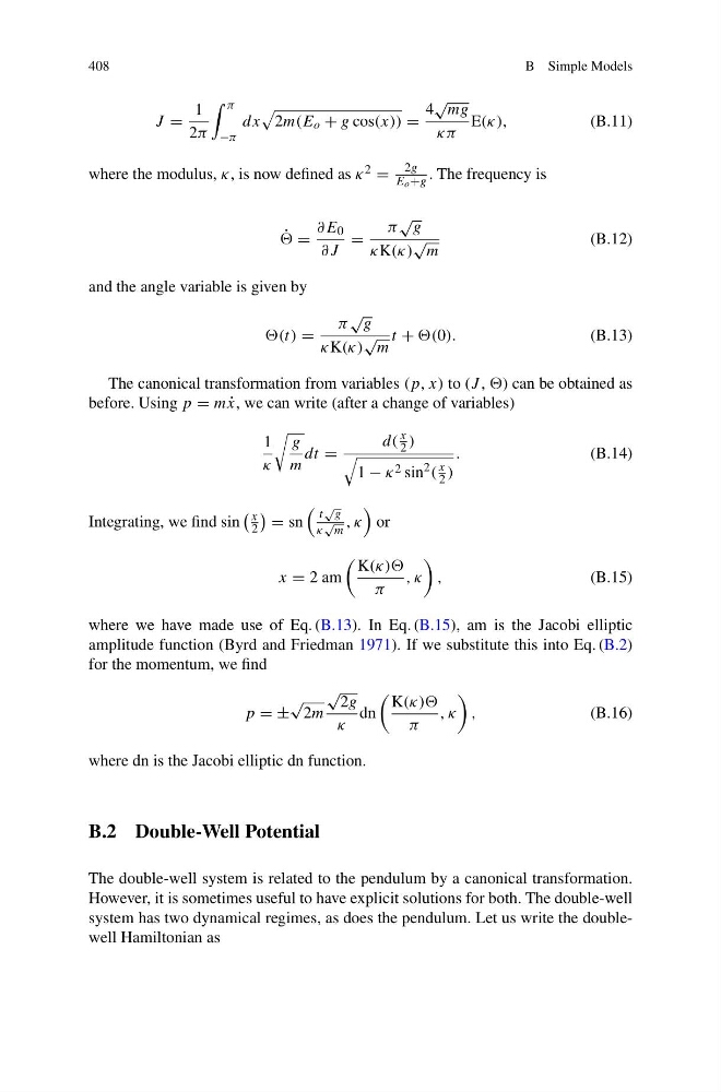
where the modulus, κ, is now defined as κ 2 =
2g
E o +g . The frequency is
˙
=
∂E 0
∂J
=
π
√ g
κK(κ)
√
m
(B.12)
and the angle variable is given by
=
π
√ g
κK(κ)
√
m
t + (0).
(B.13)
The canonical transformation from variables (p, x) to (J , ) can be obtained as
before. Using p = m ˙
x, we can write (after a change of variables)
1
κ
g
m
dt =
d(
x
2 )
1 − κ 2 sin
2 (
x
2 )
.
(B.14)
Integrating, we find sin
x
2
= sn
t
√ g
κ
√
m
, κ
or
x = 2 am
K(κ))
π
, κ
,
(B.15)
where we have made use of Eq. (B.13). In Eq. (B.15), am is the Jacobi elliptic
amplitude function (Byrd and Friedman 1971). If we substitute this into Eq. (B.2)
for the momentum, we find
p = ±
√
2m
√
2g
κ
dn
K(κ))
π
, κ
,
(B.16)
where dn is the Jacobi elliptic dn function.
B.2 Double-Well Potential
The double-well system is related to the pendulum by a canonical transformation.
However, it is sometimes useful to have explicit solutions for both. The double-well
system has two dynamical regimes, as does the pendulum. Let us write the doublewell Hamiltonian as
B Simple Models
J =
1
2π
π
−π
dx
2m(E o + g cos(x)) =
4
√ mg
κπ
E(κ),
(B.11)
where the modulus, κ, is now defined as κ 2 =
2g
E o +g . The frequency is
˙
=
∂E 0
∂J
=
π
√ g
κK(κ)
√
m
(B.12)
and the angle variable is given by
=
π
√ g
κK(κ)
√
m
t + (0).
(B.13)
The canonical transformation from variables (p, x) to (J , ) can be obtained as
before. Using p = m ˙
x, we can write (after a change of variables)
1
κ
g
m
dt =
d(
x
2 )
1 − κ 2 sin
2 (
x
2 )
.
(B.14)
Integrating, we find sin
x
2
= sn
t
√ g
κ
√
m
, κ
or
x = 2 am
K(κ))
π
, κ
,
(B.15)
where we have made use of Eq. (B.13). In Eq. (B.15), am is the Jacobi elliptic
amplitude function (Byrd and Friedman 1971). If we substitute this into Eq. (B.2)
for the momentum, we find
p = ±
√
2m
√
2g
κ
dn
K(κ))
π
, κ
,
(B.16)
where dn is the Jacobi elliptic dn function.
B.2 Double-Well Potential
The double-well system is related to the pendulum by a canonical transformation.
However, it is sometimes useful to have explicit solutions for both. The double-well
system has two dynamical regimes, as does the pendulum. Let us write the doublewell Hamiltonian as