

10.2 Floquet Theory
343
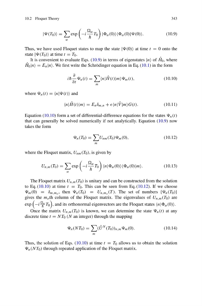
| 0 ) =
α
exp
−i
α
¯
h
T 0
| α (0) α (0)|(0).
(10.9)
Thus, we have used Floquet states to map the state |(0) at time t = 0 onto the
state | 0 ) at time t = T 0 .
It is convenient to evaluate Eqs. (10.9) in terms of eigenstates |n of ˆ
H 0 , where
ˆ
H 0 |n = E n |n. We first write the Schrödinger equation in Eq. (10.1) in the form
i ¯
h
∂
∂t
n (t) =
m
n| ˆ
H (t)|m m (t),
(10.10)
where n (t) ≡ ≡n|(t) and
n| ˆ
H (t)|m = E n δ m,n + n| ˆ
V |mG(t).
(10.11)
Equation (10.10) form a set of differential-difference equations for the states n (t)
that can generally be solved numerically if not analytically. Equation (10.9) now
takes the form
n (T 0 ) =
m
U nm (T 0 )) m (0),
(10.12)
where the Floquet matrix, U nm (T 0 ), is given by
U n,m (T 0 ) =
α
exp
−i
α
¯
h
T 0
n| α (0) α (0)|m.
(10.13)
The Floquet matrix U n,m (T 0 ) is unitary and can be constructed from the solution
to Eq. (10.10) at time t = T 0 . This can be seen from Eq. (10.12). If we choose
m (0) = δ m,m o , then n (T 0 ) = U n,m o (T ). The set of numbers { n (T 0 )}
gives the m o th column of the Floquet matrix. The eigenvalues of U n,m (T 0 ) are
exp
−i
α
¯
h T 0
, and its orthonormal eigenvectors are the Floquet states n| α (0).
Once the matrix U n,m (T 0 ) is known, we can determine the state n (t) at any
discrete time t = NT 0 (N an integer) through the mapping
n (NT 0 ) =
m
( ˆ
U
N (T 0 )) n,m m (0).
(10.14)
Thus, the solution of Eqs. (10.10) at time t = T 0 allows us to obtain the solution
n (NT 0 ) through repeated application of the Floquet matrix.
343
| 0 ) =
α
exp
−i
α
¯
h
T 0
| α (0) α (0)|(0).
(10.9)
Thus, we have used Floquet states to map the state |(0) at time t = 0 onto the
state | 0 ) at time t = T 0 .
It is convenient to evaluate Eqs. (10.9) in terms of eigenstates |n of ˆ
H 0 , where
ˆ
H 0 |n = E n |n. We first write the Schrödinger equation in Eq. (10.1) in the form
i ¯
h
∂
∂t
n (t) =
m
n| ˆ
H (t)|m m (t),
(10.10)
where n (t) ≡ ≡n|(t) and
n| ˆ
H (t)|m = E n δ m,n + n| ˆ
V |mG(t).
(10.11)
Equation (10.10) form a set of differential-difference equations for the states n (t)
that can generally be solved numerically if not analytically. Equation (10.9) now
takes the form
n (T 0 ) =
m
U nm (T 0 )) m (0),
(10.12)
where the Floquet matrix, U nm (T 0 ), is given by
U n,m (T 0 ) =
α
exp
−i
α
¯
h
T 0
n| α (0) α (0)|m.
(10.13)
The Floquet matrix U n,m (T 0 ) is unitary and can be constructed from the solution
to Eq. (10.10) at time t = T 0 . This can be seen from Eq. (10.12). If we choose
m (0) = δ m,m o , then n (T 0 ) = U n,m o (T ). The set of numbers { n (T 0 )}
gives the m o th column of the Floquet matrix. The eigenvalues of U n,m (T 0 ) are
exp
−i
α
¯
h T 0
, and its orthonormal eigenvectors are the Floquet states n| α (0).
Once the matrix U n,m (T 0 ) is known, we can determine the state n (t) at any
discrete time t = NT 0 (N an integer) through the mapping
n (NT 0 ) =
m
( ˆ
U
N (T 0 )) n,m m (0).
(10.14)
Thus, the solution of Eqs. (10.10) at time t = T 0 allows us to obtain the solution
n (NT 0 ) through repeated application of the Floquet matrix.