

320
9 Semiclassical Theory: Path Integrals
The action S γ (e) =
pdz evaluated along the γ th periodic orbit is independent of
z since it is independent of the starting point of the integration.
If we substitute the results above into Eq. (9.112) and integrate over the variables
{y i } (i = 1, . . . , d − 1), we find
g osc (e) ≈
1
i ¯
h
γ
exp
i
¯
h
S γ (e) −
iπ
2
n γ
×
dτ γ
Det
∂ 2 S γ
∂y∂y 0
Det
∂ 2 S γ
∂y∂y +
∂ 2 S γ
∂y∂y 0
+
∂ 2 S γ
∂y 0 ∂y +
∂ 2 S γ
∂y 0 ∂y 0
,
(9.122)
where we have let dτ γ =
dz γ
˙
z γ
. We can now relate the quantity under the square root
to the monodromy matrix, which provides information about the stability of orbits
in the neighborhood of a given periodic orbit.
9.6.1.1 Monodromy Matrix
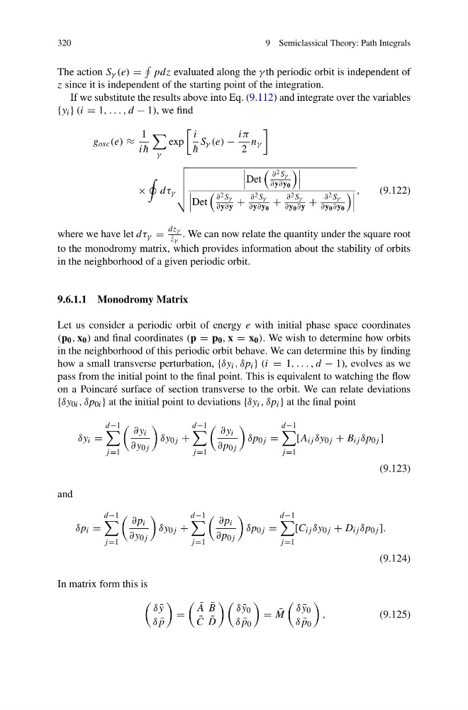
Let us consider a periodic orbit of energy e with initial phase space coordinates
(p 0 , x 0 ) and final coordinates (p = p 0 , x = x 0 ). We wish to determine how orbits
in the neighborhood of this periodic orbit behave. We can determine this by finding
how a small transverse perturbation, {δy i , δp i } (i = 1, . . . , d − 1), evolves as we
pass from the initial point to the final point. This is equivalent to watching the flow
on a Poincaré surface of section transverse to the orbit. We can relate deviations
{δy 0i , δp 0i } at the initial point to deviations {δy i , δp i } at the final point
δy i =
d−1
j =1
∂y i
∂y 0j
δy 0j +
d−1
j =1
∂y i
∂p 0j
δp 0j =
d−1
j =1
[A ij δy 0j + B ij δp 0j ]
(9.123)
and
δp i =
d−1
j =1
∂p i
∂y 0j
δy 0j +
d−1
j =1
∂p i
∂p 0j
δp 0j =
d−1
j =1
[C ij δy 0j + D ij δp 0j ].
(9.124)
In matrix form this is
δ ¯
y
δ ¯
p
=
¯
A ¯
B
¯
C ¯
D
δ ¯
y 0
δ ¯
p 0
= ¯
M
δ ¯
y 0
δ ¯
p 0
,
(9.125)
9 Semiclassical Theory: Path Integrals
The action S γ (e) =
pdz evaluated along the γ th periodic orbit is independent of
z since it is independent of the starting point of the integration.
If we substitute the results above into Eq. (9.112) and integrate over the variables
{y i } (i = 1, . . . , d − 1), we find
g osc (e) ≈
1
i ¯
h
γ
exp
i
¯
h
S γ (e) −
iπ
2
n γ
×
dτ γ
Det
∂ 2 S γ
∂y∂y 0
Det
∂ 2 S γ
∂y∂y +
∂ 2 S γ
∂y∂y 0
+
∂ 2 S γ
∂y 0 ∂y +
∂ 2 S γ
∂y 0 ∂y 0
,
(9.122)
where we have let dτ γ =
dz γ
˙
z γ
. We can now relate the quantity under the square root
to the monodromy matrix, which provides information about the stability of orbits
in the neighborhood of a given periodic orbit.
9.6.1.1 Monodromy Matrix
Let us consider a periodic orbit of energy e with initial phase space coordinates
(p 0 , x 0 ) and final coordinates (p = p 0 , x = x 0 ). We wish to determine how orbits
in the neighborhood of this periodic orbit behave. We can determine this by finding
how a small transverse perturbation, {δy i , δp i } (i = 1, . . . , d − 1), evolves as we
pass from the initial point to the final point. This is equivalent to watching the flow
on a Poincaré surface of section transverse to the orbit. We can relate deviations
{δy 0i , δp 0i } at the initial point to deviations {δy i , δp i } at the final point
δy i =
d−1
j =1
∂y i
∂y 0j
δy 0j +
d−1
j =1
∂y i
∂p 0j
δp 0j =
d−1
j =1
[A ij δy 0j + B ij δp 0j ]
(9.123)
and
δp i =
d−1
j =1
∂p i
∂y 0j
δy 0j +
d−1
j =1
∂p i
∂p 0j
δp 0j =
d−1
j =1
[C ij δy 0j + D ij δp 0j ].
(9.124)
In matrix form this is
δ ¯
y
δ ¯
p
=
¯
A ¯
B
¯
C ¯
D
δ ¯
y 0
δ ¯
p 0
= ¯
M
δ ¯
y 0
δ ¯
p 0
,
(9.125)