

9.6 Gutzwiller Trace Formula
319
where we have only noted the quantities held fixed in the derivatives of the leftmost
terms.
We wish to perform a stationary phase approximation on Eq. (9.112) by
expanding about each of the periodic orbits, γ , contained in the set β. In order
to do this, it is useful to introduce transverse coordinates, which are a special
set of orthogonal coordinates assigned to each periodic orbit such that the new
coordinates are either transverse or tangent to the given orbit. Let (x 1 , . . . , x d ) →
(z, y 1 , . . . , y d−1 ) such that the coordinate z varies along the γ th periodic orbit and
the set {y i } (i = 1, . . . , d − 1) varies perpendicular to the periodic orbit.
We now transform to coordinate frame such that {y i } = 0 on the γ th periodic
orbit. The Jacobian matrix for this transformation will be an orthogonal matrix.
Since, by definition, the velocity is directed along the orbit, we have ˙
z =0 and { ˙
y i =
0}. Thus, from Eqs. (9.114) and (9.115), we obtain
∂ 2 S γ
∂e∂z 0
= −
1
˙
z 0
and
∂ 2 S γ
∂e∂z
=
1
˙
z
,
(9.118)
while from Eqs. (9.116) and (9.117), we obtain
∂ 2 S γ
∂y i ∂z 0
=
∂ 2 S γ
∂z∂z 0
=
∂ 2 S γ
∂y 0i ∂z
= 0, (i = 1, . . . , d − 1).
(9.119)
If we make use of these new coordinates, and use the identities derived in
Eqs. (9.118) and (9.119), it is easy to show that
Det( ¯
D d,γ ) =
1
˙
z 0 ˙
z
Det
∂ 2 S γ
∂y∂y 0
,
(9.120)
where
∂ 2 S γ
∂y∂y 0
is a (d − 1) × (d − 1)-dimensional matrix consisting of derivatives of
S γ with respect to various components of y and y 0 .
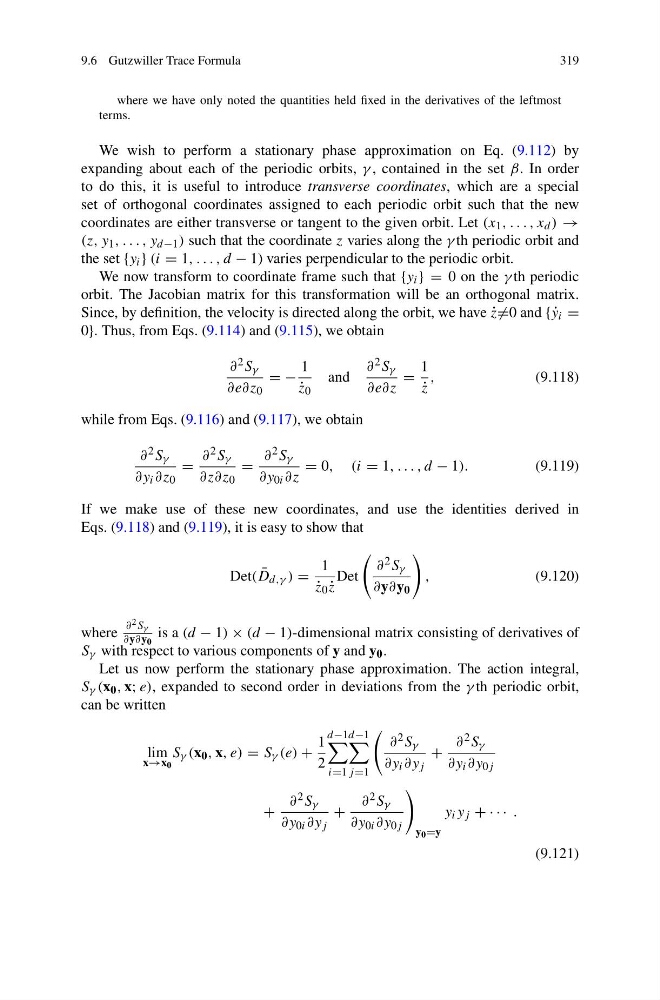
Let us now perform the stationary phase approximation. The action integral,
S γ (x 0 , x; e), expanded to second order in deviations from the γ th periodic orbit,
can be written
lim
x→x 0
S γ (x 0 , x, e) = S γ (e) +
1
2
d−1
i=1
d−1
j =1
∂ 2 S γ
∂y i ∂y j
+
∂ 2 S γ
∂y i ∂y 0j
+
∂ 2 S γ
∂y 0i ∂y j
+
∂ 2 S γ
∂y 0i ∂y 0j
y 0 =y
y i y j + · · · .
(9.121)
319
where we have only noted the quantities held fixed in the derivatives of the leftmost
terms.
We wish to perform a stationary phase approximation on Eq. (9.112) by
expanding about each of the periodic orbits, γ , contained in the set β. In order
to do this, it is useful to introduce transverse coordinates, which are a special
set of orthogonal coordinates assigned to each periodic orbit such that the new
coordinates are either transverse or tangent to the given orbit. Let (x 1 , . . . , x d ) →
(z, y 1 , . . . , y d−1 ) such that the coordinate z varies along the γ th periodic orbit and
the set {y i } (i = 1, . . . , d − 1) varies perpendicular to the periodic orbit.
We now transform to coordinate frame such that {y i } = 0 on the γ th periodic
orbit. The Jacobian matrix for this transformation will be an orthogonal matrix.
Since, by definition, the velocity is directed along the orbit, we have ˙
z =0 and { ˙
y i =
0}. Thus, from Eqs. (9.114) and (9.115), we obtain
∂ 2 S γ
∂e∂z 0
= −
1
˙
z 0
and
∂ 2 S γ
∂e∂z
=
1
˙
z
,
(9.118)
while from Eqs. (9.116) and (9.117), we obtain
∂ 2 S γ
∂y i ∂z 0
=
∂ 2 S γ
∂z∂z 0
=
∂ 2 S γ
∂y 0i ∂z
= 0, (i = 1, . . . , d − 1).
(9.119)
If we make use of these new coordinates, and use the identities derived in
Eqs. (9.118) and (9.119), it is easy to show that
Det( ¯
D d,γ ) =
1
˙
z 0 ˙
z
Det
∂ 2 S γ
∂y∂y 0
,
(9.120)
where
∂ 2 S γ
∂y∂y 0
is a (d − 1) × (d − 1)-dimensional matrix consisting of derivatives of
S γ with respect to various components of y and y 0 .
Let us now perform the stationary phase approximation. The action integral,
S γ (x 0 , x; e), expanded to second order in deviations from the γ th periodic orbit,
can be written
lim
x→x 0
S γ (x 0 , x, e) = S γ (e) +
1
2
d−1
i=1
d−1
j =1
∂ 2 S γ
∂y i ∂y j
+
∂ 2 S γ
∂y i ∂y 0j
+
∂ 2 S γ
∂y 0i ∂y j
+
∂ 2 S γ
∂y 0i ∂y 0j
y 0 =y
y i y j + · · · .
(9.121)