

9.5 Energy Green’s Function
315
Thus,
G(x 0 , x 0 ; e) =
1
i ¯
h
m
2e
(9.97)
and
¯
ρ(e) = −
1
π
Im lim
L→∞
L
−L
dx 0 G(x 0 , x 0 ; e) = lim
L→∞
2L
π ¯
h
m
2e
.
(9.98)
On the other hand,
= 2 lim
L→∞
L
−L
dx
√
2me
0
dp = lim
L→∞
4L
√
2me.
(9.99)
Therefore,
¯
ρ(e) =
1
2π ¯
h
dd
de
= lim
L→∞
2L
π ¯
h
m
2e
.
(9.100)
Thus, for this case, the two definitions of the average density of states give the same result.
Example 9.5 (Density of States for a Particle in a Potential Well)
Let us now consider a particle in a one dimensional potential well as was done in Example
9.3, but now compute the density of states (Berry and Mount 1972). We will first obtain an
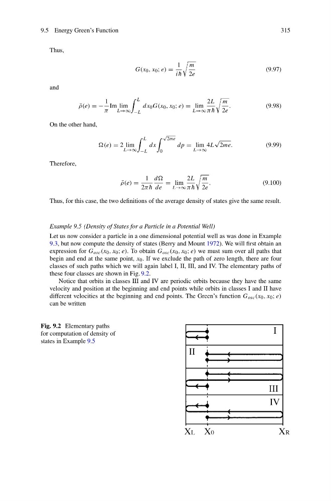
expression for G osc (x 0 , x 0 ; e). To obtain G osc (x 0 , x 0 ; e) we must sum over all paths that
begin and end at the same point, x 0 . If we exclude the path of zero length, there are four
classes of such paths which we will again label I, II, III, and IV. The elementary paths of
these four classes are shown in Fig. 9.2.
Notice that orbits in classes III and IV are periodic orbits because they have the same
velocity and position at the beginning and end points while orbits in classes I and II have
different velocities at the beginning and end points. The Green’s function G osc (x 0 , x 0 ; e)
can be written
Fig. 9.2 Elementary paths
for computation of density of
states in Example 9.5
315
Thus,
G(x 0 , x 0 ; e) =
1
i ¯
h
m
2e
(9.97)
and
¯
ρ(e) = −
1
π
Im lim
L→∞
L
−L
dx 0 G(x 0 , x 0 ; e) = lim
L→∞
2L
π ¯
h
m
2e
.
(9.98)
On the other hand,
= 2 lim
L→∞
L
−L
dx
√
2me
0
dp = lim
L→∞
4L
√
2me.
(9.99)
Therefore,
¯
ρ(e) =
1
2π ¯
h
dd
de
= lim
L→∞
2L
π ¯
h
m
2e
.
(9.100)
Thus, for this case, the two definitions of the average density of states give the same result.
Example 9.5 (Density of States for a Particle in a Potential Well)
Let us now consider a particle in a one dimensional potential well as was done in Example
9.3, but now compute the density of states (Berry and Mount 1972). We will first obtain an
expression for G osc (x 0 , x 0 ; e). To obtain G osc (x 0 , x 0 ; e) we must sum over all paths that
begin and end at the same point, x 0 . If we exclude the path of zero length, there are four
classes of such paths which we will again label I, II, III, and IV. The elementary paths of
these four classes are shown in Fig. 9.2.
Notice that orbits in classes III and IV are periodic orbits because they have the same
velocity and position at the beginning and end points while orbits in classes I and II have
different velocities at the beginning and end points. The Green’s function G osc (x 0 , x 0 ; e)
can be written
Fig. 9.2 Elementary paths
for computation of density of
states in Example 9.5