

9.5 Energy Green’s Function
313
G osc (x 0 , x f ; e) =
1
i ¯
h
m
2(e − V (x 0 ))
1/4
m
2(e − V (x f ))
1/4
× e
i
¯
h S(e)
∞
n=0
e
i
¯
h 2nS(e) e
−inπ
×
e
−
i
¯
h (S L,0 +S f,R ) + e
−
i
¯
h (−S L,0 +S f,R ) e
−
iπ
2
+e
+
i
¯
h (−S L,0 +S f,R ) e
−
iπ
2 + e
i
¯
h (S L,0 +S f,R ) e
−iπ
.
(9.87)
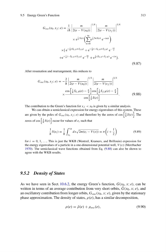
After resumation and rearrangement, this reduces to
G osc (x 0 , x f ; e) = −
2
¯
h
m
2(e − V (x 0 ))
1/4
m
2(e − V (x f ))
1/4
×
cos
1
¯
h S L,0 (e) −
π
4
cos
1
¯
h S f,R (e) −
π
4
cos
1
¯
h S(e)
.
(9.88)
The contribution to the Green’s function for x f < x 0 is given by a similar analysis.
We can obtain a semiclassical expression for energy eigenvalues of this system. These
are given by the poles of G osc (x 0 , x f ; e) and therefore by the zeros of cos
1
¯
h S(e)
. The
zeros of cos
1
¯
h S(e)
occur for values of e i such that
1
¯
h
S(e i ) =
1
¯
h
x R
x L
dx
2m(e i − V (x)) = π
i +
1
2
(9.89)
for i = 0, 1, . . .. This is just the WKB (Wentzel, Kramers, and Brillouin) expression for
the energy eigenvalues of a particle in a one-dimensional potential well, V (x) (Merzbacher
1970). The semiclassical wave functions obtained from Eq. (9.88) can also be shown to
agree with the WKB results.
9.5.2 Density of States
As we have seen in Sect. 10.6.2, the energy Green’s function, G(x 0 , x; e), can be
written in terms of an average contribution from very short orbits, ¯
G(x 0 , x; e), and
an oscillatory contribution from longer orbits, G osc (x 0 , x; e), given by the stationary
phase approximation. The density of states, ρ(e), has a similar decomposition,
ρ(e) = ¯
ρ(e) + ρ osc (e),
(9.90)
313
G osc (x 0 , x f ; e) =
1
i ¯
h
m
2(e − V (x 0 ))
1/4
m
2(e − V (x f ))
1/4
× e
i
¯
h S(e)
∞
n=0
e
i
¯
h 2nS(e) e
−inπ
×
e
−
i
¯
h (S L,0 +S f,R ) + e
−
i
¯
h (−S L,0 +S f,R ) e
−
iπ
2
+e
+
i
¯
h (−S L,0 +S f,R ) e
−
iπ
2 + e
i
¯
h (S L,0 +S f,R ) e
−iπ
.
(9.87)
After resumation and rearrangement, this reduces to
G osc (x 0 , x f ; e) = −
2
¯
h
m
2(e − V (x 0 ))
1/4
m
2(e − V (x f ))
1/4
×
cos
1
¯
h S L,0 (e) −
π
4
cos
1
¯
h S f,R (e) −
π
4
cos
1
¯
h S(e)
.
(9.88)
The contribution to the Green’s function for x f < x 0 is given by a similar analysis.
We can obtain a semiclassical expression for energy eigenvalues of this system. These
are given by the poles of G osc (x 0 , x f ; e) and therefore by the zeros of cos
1
¯
h S(e)
. The
zeros of cos
1
¯
h S(e)
occur for values of e i such that
1
¯
h
S(e i ) =
1
¯
h
x R
x L
dx
2m(e i − V (x)) = π
i +
1
2
(9.89)
for i = 0, 1, . . .. This is just the WKB (Wentzel, Kramers, and Brillouin) expression for
the energy eigenvalues of a particle in a one-dimensional potential well, V (x) (Merzbacher
1970). The semiclassical wave functions obtained from Eq. (9.88) can also be shown to
agree with the WKB results.
9.5.2 Density of States
As we have seen in Sect. 10.6.2, the energy Green’s function, G(x 0 , x; e), can be
written in terms of an average contribution from very short orbits, ¯
G(x 0 , x; e), and
an oscillatory contribution from longer orbits, G osc (x 0 , x; e), given by the stationary
phase approximation. The density of states, ρ(e), has a similar decomposition,
ρ(e) = ¯
ρ(e) + ρ osc (e),
(9.90)