

9.5 Energy Green’s Function
311
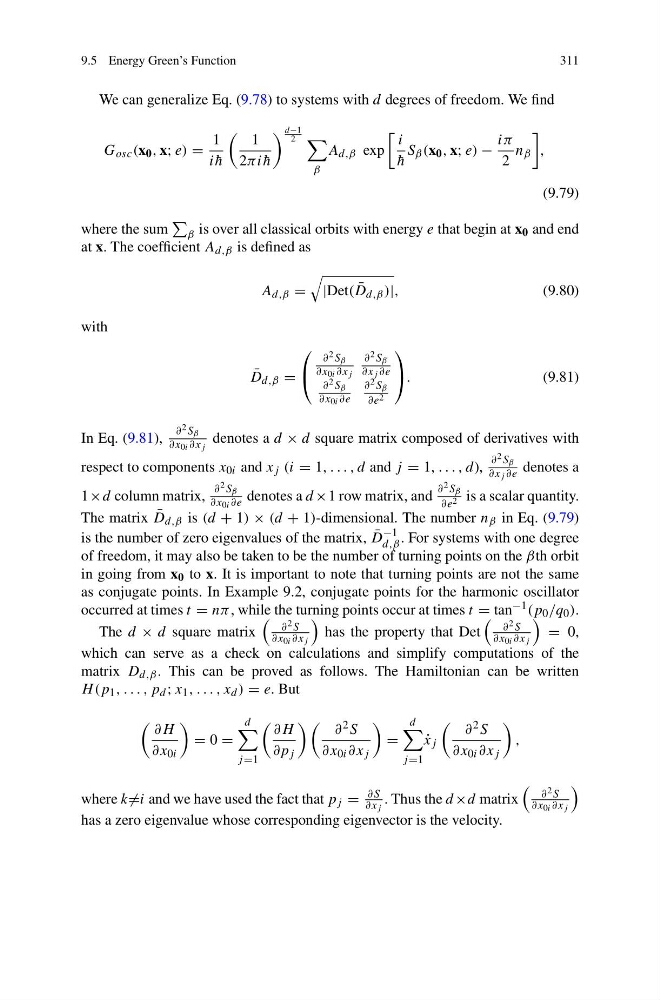
We can generalize Eq. (9.78) to systems with d degrees of freedom. We find
G osc (x 0 , x; e) =
1
i ¯
h
1
2πi ¯
h
d−1
2
β
A d,β exp
i
¯
h
S β (x 0 , x; e) −
iπ
2
n β
,
(9.79)
where the sum
β is over all classical orbits with energy e that begin at x 0 and end
at x. The coefficient A d,β is defined as
A d,β =
|Det( ¯
D d,β )|,
(9.80)
with
¯
D d,β =
⎛
⎝
∂ 2 S β
∂x 0i ∂x j
∂ 2 S β
∂x j ∂e
∂ 2 S β
∂x 0i ∂e
∂ 2 S β
∂e 2
⎞
⎠ .
(9.81)
In Eq. (9.81),
∂ 2 S β
∂x 0i ∂x j
denotes a d × d square matrix composed of derivatives with
respect to components x 0i and x j (i = 1, . . . , d and j = 1, . . . , d),
∂ 2 S β
∂x j ∂e denotes a
1×d column matrix,
∂ 2 S β
∂x 0i ∂e denotes a d ×1 row matrix, and
∂ 2 S β
∂e 2 is a scalar quantity.
The matrix ¯
D d,β is (d + 1) × (d + 1)-dimensional. The number n β in Eq. (9.79)
is the number of zero eigenvalues of the matrix, ¯
D
−1
d,β . For systems with one degree
of freedom, it may also be taken to be the number of turning points on the βth orbit
in going from x 0 to x. It is important to note that turning points are not the same
as conjugate points. In Example 9.2, conjugate points for the harmonic oscillator
occurred at times t = nπ , while the turning points occur at times t = tan −1 (p 0 /q 0 ).
The d × d square matrix
∂ 2 S
∂x 0i ∂x j
has the property that Det
∂ 2 S
∂x 0i ∂x j
= 0,
which can serve as a check on calculations and simplify computations of the
matrix D d,β . This can be proved as follows. The Hamiltonian can be written
H (p 1 , . . . , p d ; x 1 , . . . , x d ) = e. But
∂H
∂x 0i
= 0 =
d
j =1
∂H
∂p j
∂ 2 S
∂x 0i ∂x j
=
d
j =1
˙
x j
∂ 2 S
∂x 0i ∂x j
,
where k =i and we have used the fact that p j =
∂S
∂x j
. Thus the d ×d matrix
∂ 2 S
∂x 0i ∂x j
has a zero eigenvalue whose corresponding eigenvector is the velocity.
311
We can generalize Eq. (9.78) to systems with d degrees of freedom. We find
G osc (x 0 , x; e) =
1
i ¯
h
1
2πi ¯
h
d−1
2
β
A d,β exp
i
¯
h
S β (x 0 , x; e) −
iπ
2
n β
,
(9.79)
where the sum
β is over all classical orbits with energy e that begin at x 0 and end
at x. The coefficient A d,β is defined as
A d,β =
|Det( ¯
D d,β )|,
(9.80)
with
¯
D d,β =
⎛
⎝
∂ 2 S β
∂x 0i ∂x j
∂ 2 S β
∂x j ∂e
∂ 2 S β
∂x 0i ∂e
∂ 2 S β
∂e 2
⎞
⎠ .
(9.81)
In Eq. (9.81),
∂ 2 S β
∂x 0i ∂x j
denotes a d × d square matrix composed of derivatives with
respect to components x 0i and x j (i = 1, . . . , d and j = 1, . . . , d),
∂ 2 S β
∂x j ∂e denotes a
1×d column matrix,
∂ 2 S β
∂x 0i ∂e denotes a d ×1 row matrix, and
∂ 2 S β
∂e 2 is a scalar quantity.
The matrix ¯
D d,β is (d + 1) × (d + 1)-dimensional. The number n β in Eq. (9.79)
is the number of zero eigenvalues of the matrix, ¯
D
−1
d,β . For systems with one degree
of freedom, it may also be taken to be the number of turning points on the βth orbit
in going from x 0 to x. It is important to note that turning points are not the same
as conjugate points. In Example 9.2, conjugate points for the harmonic oscillator
occurred at times t = nπ , while the turning points occur at times t = tan −1 (p 0 /q 0 ).
The d × d square matrix
∂ 2 S
∂x 0i ∂x j
has the property that Det
∂ 2 S
∂x 0i ∂x j
= 0,
which can serve as a check on calculations and simplify computations of the
matrix D d,β . This can be proved as follows. The Hamiltonian can be written
H (p 1 , . . . , p d ; x 1 , . . . , x d ) = e. But
∂H
∂x 0i
= 0 =
d
j =1
∂H
∂p j
∂ 2 S
∂x 0i ∂x j
=
d
j =1
˙
x j
∂ 2 S
∂x 0i ∂x j
,
where k =i and we have used the fact that p j =
∂S
∂x j
. Thus the d ×d matrix
∂ 2 S
∂x 0i ∂x j
has a zero eigenvalue whose corresponding eigenvector is the velocity.