

9.4 Semiclassical Approximation
303
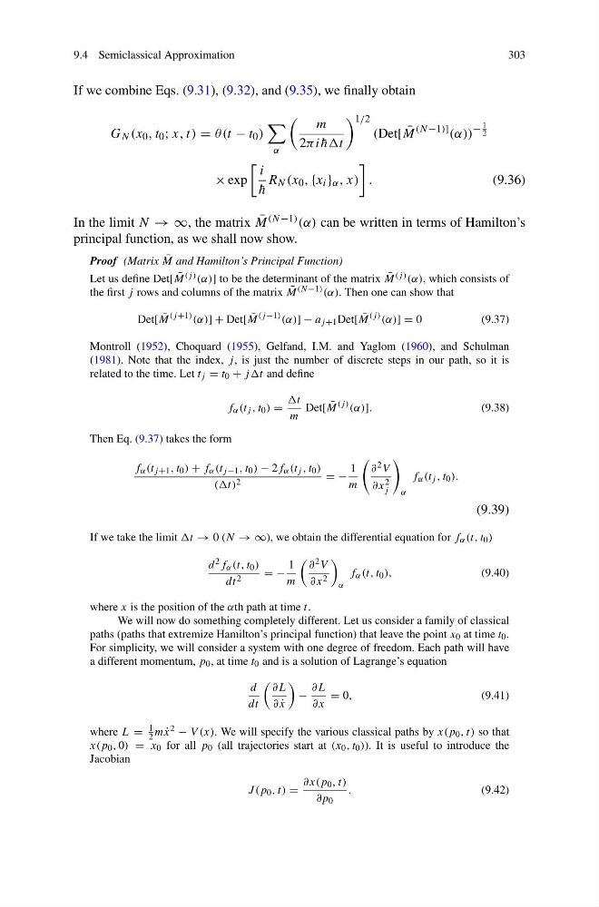
If we combine Eqs. (9.31), (9.32), and (9.35), we finally obtain
G N (x 0 , t 0 ; x, t) = θ(t − t 0 )
α
m
2πi ¯
hht
1/2
(Det[ ¯
M
(N −1)] (α))
−
1
2
× exp
i
¯
h
R N (x 0 , {x i } α , x)
.
(9.36)
In the limit N → ∞, the matrix ¯
M (N −1) (α) can be written in terms of Hamilton’s
principal function, as we shall now show.
Proof (Matrix ¯
M and Hamilton’s Principal Function)
Let us define Det[ ¯
M (j ) (α)] to be the determinant of the matrix ¯
M (j ) (α), which consists of
the first j rows and columns of the matrix ¯
M (N −1) (α). Then one can show that
Det[ ¯
M
(j +1) (α)] + Det[ ¯
M
(j −1) (α)] − a j +1 Det[ ¯
M
(j ) (α)] = 0
(9.37)
Montroll (1952), Choquard (1955), Gelfand, I.M. and Yaglom (1960), and Schulman
(1981). Note that the index, j , is just the number of discrete steps in our path, so it is
related to the time. Let t j = t 0 + jjt and define
f α (t j , t 0 ) =
t
m
Det[ ¯
M
(j ) (α)].
(9.38)
Then Eq. (9.37) takes the form
f α (t j +1 , t 0 ) + f α (t j −1 , t 0 ) − 2f α (t j , t 0 )
((t) 2
= −
1
m
∂ 2 V
∂x 2
j
α
f α (t j , t 0 ).
(9.39)
If we take the limit t → 0 (N → ∞), we obtain the differential equation for f α (t, t 0 )
d 2 f α (t, t 0 )
dt 2
= −
1
m
∂ 2 V
∂x 2
α
f α (t, t 0 ),
(9.40)
where x is the position of the αth path at time t.
We will now do something completely different. Let us consider a family of classical
paths (paths that extremize Hamilton’s principal function) that leave the point x 0 at time t 0 .
For simplicity, we will consider a system with one degree of freedom. Each path will have
a different momentum, p 0 , at time t 0 and is a solution of Lagrange’s equation
d
dt
∂L
∂ ˙
x
−
∂L
∂x
= 0,
(9.41)
where L =
1
2 m ˙
x 2 − V (x). We will specify the various classical paths by x(p 0 , t) so that
x(p 0 , 0) = x 0 for all p 0 (all trajectories start at (x 0 , t 0 )). It is useful to introduce the
Jacobian
J (p 0 , t) =
∂x(p 0 , t)
∂p 0
.
(9.42)
303
If we combine Eqs. (9.31), (9.32), and (9.35), we finally obtain
G N (x 0 , t 0 ; x, t) = θ(t − t 0 )
α
m
2πi ¯
hht
1/2
(Det[ ¯
M
(N −1)] (α))
−
1
2
× exp
i
¯
h
R N (x 0 , {x i } α , x)
.
(9.36)
In the limit N → ∞, the matrix ¯
M (N −1) (α) can be written in terms of Hamilton’s
principal function, as we shall now show.
Proof (Matrix ¯
M and Hamilton’s Principal Function)
Let us define Det[ ¯
M (j ) (α)] to be the determinant of the matrix ¯
M (j ) (α), which consists of
the first j rows and columns of the matrix ¯
M (N −1) (α). Then one can show that
Det[ ¯
M
(j +1) (α)] + Det[ ¯
M
(j −1) (α)] − a j +1 Det[ ¯
M
(j ) (α)] = 0
(9.37)
Montroll (1952), Choquard (1955), Gelfand, I.M. and Yaglom (1960), and Schulman
(1981). Note that the index, j , is just the number of discrete steps in our path, so it is
related to the time. Let t j = t 0 + jjt and define
f α (t j , t 0 ) =
t
m
Det[ ¯
M
(j ) (α)].
(9.38)
Then Eq. (9.37) takes the form
f α (t j +1 , t 0 ) + f α (t j −1 , t 0 ) − 2f α (t j , t 0 )
((t) 2
= −
1
m
∂ 2 V
∂x 2
j
α
f α (t j , t 0 ).
(9.39)
If we take the limit t → 0 (N → ∞), we obtain the differential equation for f α (t, t 0 )
d 2 f α (t, t 0 )
dt 2
= −
1
m
∂ 2 V
∂x 2
α
f α (t, t 0 ),
(9.40)
where x is the position of the αth path at time t.
We will now do something completely different. Let us consider a family of classical
paths (paths that extremize Hamilton’s principal function) that leave the point x 0 at time t 0 .
For simplicity, we will consider a system with one degree of freedom. Each path will have
a different momentum, p 0 , at time t 0 and is a solution of Lagrange’s equation
d
dt
∂L
∂ ˙
x
−
∂L
∂x
= 0,
(9.41)
where L =
1
2 m ˙
x 2 − V (x). We will specify the various classical paths by x(p 0 , t) so that
x(p 0 , 0) = x 0 for all p 0 (all trajectories start at (x 0 , t 0 )). It is useful to introduce the
Jacobian
J (p 0 , t) =
∂x(p 0 , t)
∂p 0
.
(9.42)