

274
8 Manifestations of Chaos in Quantum Scattering Processes
in Appendix G). Then in Sect. 8.6.2, we introduce the Lorentzian Orthogonal
Ensemble (OE), which is the key to relating COE to GOE, and we discuss
some relevant features of the OE. In Sect. 8.6.3, we discuss the relation between
COE and OE. Then finally, in Sect. 8.6.4, we describe the particular conditions
under which a scattering system, whose dynamics is governed by a GOE random
Hamiltonian matrix, will give a scattering matrix that is a member of the COE.
8.6.1 Circular Orthogonal Ensembles
The circular ensembles were introduced by Dyson (1962a,b,c) to aid in the analysis
of nuclear scattering data. The circular ensembles are based upon the statistical
properties of N ×N unitary matrices rather than Hermitian matrices, since most
scattering properties are determined by the unitary S-matrix (scattering matrix),
which connects incoming states to outgoing states in the scattering process.
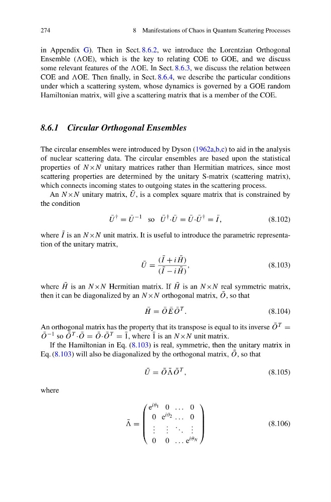
An N ×N unitary matrix, ¯
U , is a complex square matrix that is constrained by
the condition
¯
U
†
= ¯
U
−1 so ¯
U
†
· ¯
U = ¯
U · ¯
U
†
= ¯
I ,
(8.102)
where ¯
I is an N ×N unit matrix. It is useful to introduce the parametric representation of the unitary matrix,
¯
U =
( ¯
I + i ¯
H )
( ¯
I − i ¯
H )
,
(8.103)
where ¯
H is an N ×N Hermitian matrix. If ¯
H is an N ×N real symmetric matrix,
then it can be diagonalized by an N×N orthogonal matrix, ¯
O, so that
¯
H = ¯
O ¯
E ¯
O
T .
(8.104)
An orthogonal matrix has the property that its transpose is equal to its inverse ¯
O T =
¯
O −1 so ¯
O T · ¯
O = ¯
O· ¯
O T = ¯
1, where ¯
1 is an N×N unit matrix.
If the Hamiltonian in Eq. (8.103) is real, symmetric, then the unitary matrix in
Eq. (8.103) will also be diagonalized by the orthogonal matrix, ¯
O, so that
¯
U = ¯
O ¯
¯
O
T ,
(8.105)
where
¯
=
⎛
⎜
⎜
⎜
⎝
e iθ 1 0 . . . 0
0 e iθ 2 . . . 0
. . .
. . .
. . .
. . .
0 0 . . . e iθ N
⎞
⎟
⎟
⎟
⎠
(8.106)
8 Manifestations of Chaos in Quantum Scattering Processes
in Appendix G). Then in Sect. 8.6.2, we introduce the Lorentzian Orthogonal
Ensemble (OE), which is the key to relating COE to GOE, and we discuss
some relevant features of the OE. In Sect. 8.6.3, we discuss the relation between
COE and OE. Then finally, in Sect. 8.6.4, we describe the particular conditions
under which a scattering system, whose dynamics is governed by a GOE random
Hamiltonian matrix, will give a scattering matrix that is a member of the COE.
8.6.1 Circular Orthogonal Ensembles
The circular ensembles were introduced by Dyson (1962a,b,c) to aid in the analysis
of nuclear scattering data. The circular ensembles are based upon the statistical
properties of N ×N unitary matrices rather than Hermitian matrices, since most
scattering properties are determined by the unitary S-matrix (scattering matrix),
which connects incoming states to outgoing states in the scattering process.
An N ×N unitary matrix, ¯
U , is a complex square matrix that is constrained by
the condition
¯
U
†
= ¯
U
−1 so ¯
U
†
· ¯
U = ¯
U · ¯
U
†
= ¯
I ,
(8.102)
where ¯
I is an N ×N unit matrix. It is useful to introduce the parametric representation of the unitary matrix,
¯
U =
( ¯
I + i ¯
H )
( ¯
I − i ¯
H )
,
(8.103)
where ¯
H is an N ×N Hermitian matrix. If ¯
H is an N ×N real symmetric matrix,
then it can be diagonalized by an N×N orthogonal matrix, ¯
O, so that
¯
H = ¯
O ¯
E ¯
O
T .
(8.104)
An orthogonal matrix has the property that its transpose is equal to its inverse ¯
O T =
¯
O −1 so ¯
O T · ¯
O = ¯
O· ¯
O T = ¯
1, where ¯
1 is an N×N unit matrix.
If the Hamiltonian in Eq. (8.103) is real, symmetric, then the unitary matrix in
Eq. (8.103) will also be diagonalized by the orthogonal matrix, ¯
O, so that
¯
U = ¯
O ¯
¯
O
T ,
(8.105)
where
¯
=
⎛
⎜
⎜
⎜
⎝
e iθ 1 0 . . . 0
0 e iθ 2 . . . 0
. . .
. . .
. . .
. . .
0 0 . . . e iθ N
⎞
⎟
⎟
⎟
⎠
(8.106)