

264
8 Manifestations of Chaos in Quantum Scattering Processes
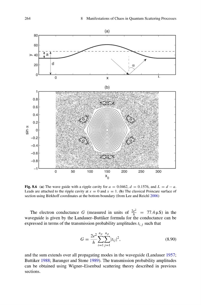
Fig. 8.6 (a) The wave guide with a ripple cavity for a = 0.0462, d = 0.1576, and L = d − a.
Leads are attached to the ripple cavity at x = 0 and x = 1. (b) The classical Poincare surface of
section using Birkhoff coordinates at the bottom boundary (from Lee and Reichl 2006)
The electron conductance G (measured in units of
2e 2
h
= 77.4 µS) in the
waveguide is given by the Landauer–Buttiker formula for the conductance can be
expressed in terms of the transmission probability amplitudes t i,j such that
G =
2e 2
h
n p
i=1
n p
j =1
|t ij |
2 ,
(8.90)
and the sum extends over all propagating modes in the waveguide (Landauer 1957;
Buttiker 1988; Baranger and Stone 1989). The transmission probability amplitudes
can be obtained using Wigner–Eisenbud scattering theory described in previous
sections.
8 Manifestations of Chaos in Quantum Scattering Processes
Fig. 8.6 (a) The wave guide with a ripple cavity for a = 0.0462, d = 0.1576, and L = d − a.
Leads are attached to the ripple cavity at x = 0 and x = 1. (b) The classical Poincare surface of
section using Birkhoff coordinates at the bottom boundary (from Lee and Reichl 2006)
The electron conductance G (measured in units of
2e 2
h
= 77.4 µS) in the
waveguide is given by the Landauer–Buttiker formula for the conductance can be
expressed in terms of the transmission probability amplitudes t i,j such that
G =
2e 2
h
n p
i=1
n p
j =1
|t ij |
2 ,
(8.90)
and the sum extends over all propagating modes in the waveguide (Landauer 1957;
Buttiker 1988; Baranger and Stone 1989). The transmission probability amplitudes
can be obtained using Wigner–Eisenbud scattering theory described in previous
sections.