

8.4 Wigner–Smith and Partial Delay Times
259
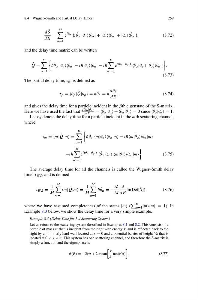
d ˆ
S
dE
=
M
α=1
e
iθ α {i ˙
θ α |θ α θ α | + | ˙
θ α θ α | + |θ α ˙
θ α |},
(8.72)
and the delay time matrix can be written
ˆ
Q =
M
α=1
¯
h ˙
θ α |θ α θ α | − i ¯
h| ˙
θ α θ α | − i ¯
h
M
α =1
e
i(θ α −θ α )
˙
θ α |θ α |θ α θ α |
.
(8.73)
The partial delay time, τ β , is defined as
τ β = =θ β | ˆ
Q|θ β = ¯
h ˙
θ β = ¯
h
dθ β
dE
,
(8.74)
and gives the delay time for a particle incident in the βth eigenstate of the S-matrix.
Here we have used the fact that
dθ α |θ α
dE
= = ˙
θ α |θ α + +θ α | ˙
θ α = 0 since θ α |θ α = 1.
Let τ m denote the delay time for a particle incident in the mth scattering channel,
where
τ m = =m| ˆ
Q|m =
M
α=1
¯
h ˙
θ α m|θ α θ α |m − i ¯
hm| ˙
θ α θ α |m
−i ¯
h
M
α =1
e
i(θ α −θ α )
˙
θ α |θ α m|θ α θ α |m
(8.75)
The average delay time for all the channels is called the Wigner–Smith delay
time, τ W S , and is defined
τ W S =
1
M
M
m=1
m| ˆ
Q|m =
1
M
M
α=1
¯
h ˙
θ α = −
i ¯
h
M
d
dE
ln(Det[ ˆ
S]),
(8.76)
where we have assumed completeness of the states |m (
M
m=1 |mm| = 1). In
Example 8.3 below, we show the delay time for a very simple example.
Example 8.3 (Delay Time for 1-d Scattering System)
Let us return to the scattering system described in Examples 8.1 and 8.2. This consists of a
particle of mass m that is incident from the right with energy E and is reflected back to the
right by an infinitely hard wall located at x = 0 and a potential barrier of height V 0 that is
located at 0 < x < a. This system has one scattering channel, and therefore the S-matrix is
simply a function and the eigenphase is
θ(E) = −2ka + 2arctan
k
k tan(k
a)
,
(8.77)
259
d ˆ
S
dE
=
M
α=1
e
iθ α {i ˙
θ α |θ α θ α | + | ˙
θ α θ α | + |θ α ˙
θ α |},
(8.72)
and the delay time matrix can be written
ˆ
Q =
M
α=1
¯
h ˙
θ α |θ α θ α | − i ¯
h| ˙
θ α θ α | − i ¯
h
M
α =1
e
i(θ α −θ α )
˙
θ α |θ α |θ α θ α |
.
(8.73)
The partial delay time, τ β , is defined as
τ β = =θ β | ˆ
Q|θ β = ¯
h ˙
θ β = ¯
h
dθ β
dE
,
(8.74)
and gives the delay time for a particle incident in the βth eigenstate of the S-matrix.
Here we have used the fact that
dθ α |θ α
dE
= = ˙
θ α |θ α + +θ α | ˙
θ α = 0 since θ α |θ α = 1.
Let τ m denote the delay time for a particle incident in the mth scattering channel,
where
τ m = =m| ˆ
Q|m =
M
α=1
¯
h ˙
θ α m|θ α θ α |m − i ¯
hm| ˙
θ α θ α |m
−i ¯
h
M
α =1
e
i(θ α −θ α )
˙
θ α |θ α m|θ α θ α |m
(8.75)
The average delay time for all the channels is called the Wigner–Smith delay
time, τ W S , and is defined
τ W S =
1
M
M
m=1
m| ˆ
Q|m =
1
M
M
α=1
¯
h ˙
θ α = −
i ¯
h
M
d
dE
ln(Det[ ˆ
S]),
(8.76)
where we have assumed completeness of the states |m (
M
m=1 |mm| = 1). In
Example 8.3 below, we show the delay time for a very simple example.
Example 8.3 (Delay Time for 1-d Scattering System)
Let us return to the scattering system described in Examples 8.1 and 8.2. This consists of a
particle of mass m that is incident from the right with energy E and is reflected back to the
right by an infinitely hard wall located at x = 0 and a potential barrier of height V 0 that is
located at 0 < x < a. This system has one scattering channel, and therefore the S-matrix is
simply a function and the eigenphase is
θ(E) = −2ka + 2arctan
k
k tan(k
a)
,
(8.77)