

244
8 Manifestations of Chaos in Quantum Scattering Processes
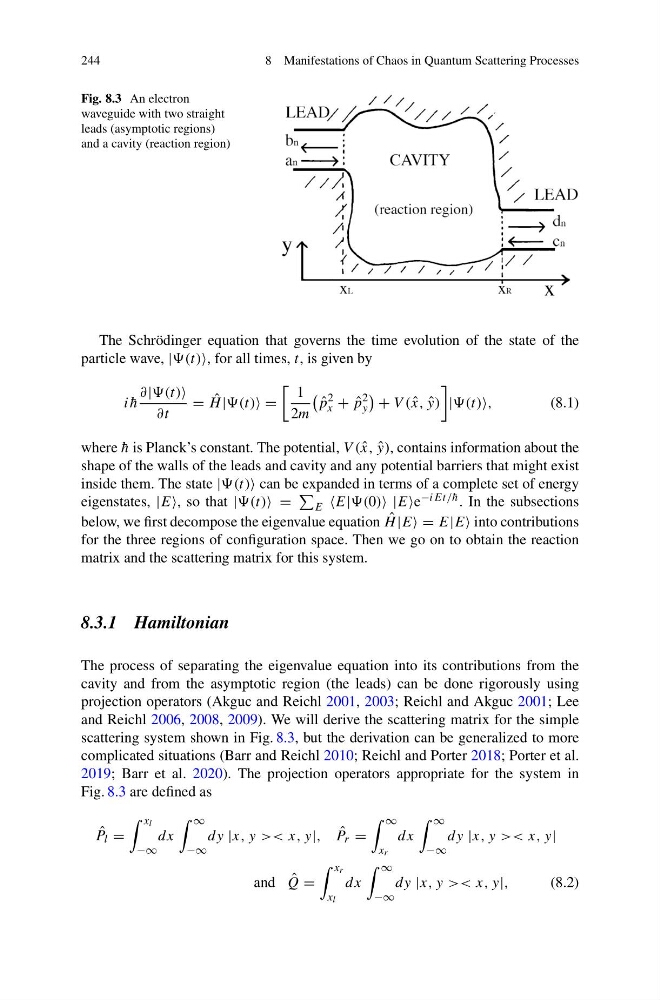
Fig. 8.3 An electron
waveguide with two straight
leads (asymptotic regions)
and a cavity (reaction region)
The Schrödinger equation that governs the time evolution of the state of the
particle wave, | for all times, t, is given by
i ¯
h
∂|
∂t
= ˆ
H |(t) =
1
2m
ˆ
p
2
x + ˆ
p
2
y
+ V ( ˆ
x, ˆ
y)
|(t)
(8.1)
where ¯
h is Planck’s constant. The potential, V ( ˆ
x, ˆ
y), contains information about the
shape of the walls of the leads and cavity and any potential barriers that might exist
inside them. The state | can be expanded in terms of a complete set of energy
eigenstates, |E, so that |(t) =
E |E −iEt/¯ h . In the subsections
below, we first decompose the eigenvalue equation ˆ
H |E = E|E into contributions
for the three regions of configuration space. Then we go on to obtain the reaction
matrix and the scattering matrix for this system.
8.3.1 Hamiltonian
The process of separating the eigenvalue equation into its contributions from the
cavity and from the asymptotic region (the leads) can be done rigorously using
projection operators (Akguc and Reichl 2001, 2003; Reichl and Akguc 2001; Lee
and Reichl 2006, 2008, 2009). We will derive the scattering matrix for the simple
scattering system shown in Fig. 8.3, but the derivation can be generalized to more
complicated situations (Barr and Reichl 2010; Reichl and Porter 2018; Porter et al.
2019; Barr et al. 2020). The projection operators appropriate for the system in
Fig. 8.3 are defined as
ˆ
P l =
x l
−∞
dx
∞
−∞
dy |x, y >< x, y|, ˆ
P r =
∞
x r
dx
∞
−∞
dy |x, y >< x, y|
and ˆ
Q =
x r
x l
dx
∞
−∞
dy |x, y >< x, y|,
(8.2)
8 Manifestations of Chaos in Quantum Scattering Processes
Fig. 8.3 An electron
waveguide with two straight
leads (asymptotic regions)
and a cavity (reaction region)
The Schrödinger equation that governs the time evolution of the state of the
particle wave, | for all times, t, is given by
i ¯
h
∂|
∂t
= ˆ
H |(t) =
1
2m
ˆ
p
2
x + ˆ
p
2
y
+ V ( ˆ
x, ˆ
y)
|(t)
(8.1)
where ¯
h is Planck’s constant. The potential, V ( ˆ
x, ˆ
y), contains information about the
shape of the walls of the leads and cavity and any potential barriers that might exist
inside them. The state | can be expanded in terms of a complete set of energy
eigenstates, |E, so that |(t) =
E |E −iEt/¯ h . In the subsections
below, we first decompose the eigenvalue equation ˆ
H |E = E|E into contributions
for the three regions of configuration space. Then we go on to obtain the reaction
matrix and the scattering matrix for this system.
8.3.1 Hamiltonian
The process of separating the eigenvalue equation into its contributions from the
cavity and from the asymptotic region (the leads) can be done rigorously using
projection operators (Akguc and Reichl 2001, 2003; Reichl and Akguc 2001; Lee
and Reichl 2006, 2008, 2009). We will derive the scattering matrix for the simple
scattering system shown in Fig. 8.3, but the derivation can be generalized to more
complicated situations (Barr and Reichl 2010; Reichl and Porter 2018; Porter et al.
2019; Barr et al. 2020). The projection operators appropriate for the system in
Fig. 8.3 are defined as
ˆ
P l =
x l
−∞
dx
∞
−∞
dy |x, y >< x, y|, ˆ
P r =
∞
x r
dx
∞
−∞
dy |x, y >< x, y|
and ˆ
Q =
x r
x l
dx
∞
−∞
dy |x, y >< x, y|,
(8.2)