

222
7 Bounded Quantum Systems
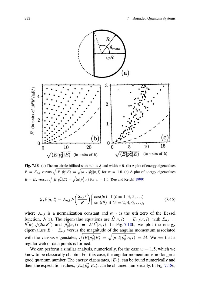
Fig. 7.18 (a) The cut-circle billiard with radius R and width wR. (b) A plot of energy eigenvalues
E = E n,l versus
ˆ
p 2
θ |E =
n, l| ˆ
p 2
θ |n, l for w = 1.0. (c) A plot of energy eigenvalues
E = E n versus
E| ˆ
p 2
θ |E =
n| ˆ
p 2
θ |n for w = 1.5 (Ree and Reichl 1999)
r, θ |n, l = A n,l J l
α n,l r
R
cos(lθ ) if (( = 1, 3, 5, . . .)
sin(lθ ) if (( = 2, 4, 6, . . .),
(7.45)
where A n,l is a normalization constant and α n,l is the nth zero of the Bessel
function, J l (x). The eigenvalue equations are ˆ
H |n, l = E n,l |n, l, with E n,l =
¯
h 2 α 2
n,l /(2mR 2 ) and ˆ
p 2
θ |n, l = ¯
h 2 l 2 |n, l. In Fig. 7.18b, we plot the energy
eigenvalues E = E n,l versus the magnitude of the angular momentum associated
with the various eigenstates,
E| ˆ
p 2
θ |E =
n, l| ˆ
p 2
θ |n, l = ¯
hl. We see that a
regular web of data points is formed.
We can perform a similar analysis, numerically, for the case w = 1.5, which we
know to be classically chaotic. For this case, the angular momentum is no longer a
good quantum number. The energy eigenstates, |E n , can be found numerically and
then, the expectation values, n | ˆ
p 2
θ |E n , can be obtained numerically. In Fig. 7.18c,
7 Bounded Quantum Systems
Fig. 7.18 (a) The cut-circle billiard with radius R and width wR. (b) A plot of energy eigenvalues
E = E n,l versus
ˆ
p 2
θ |E =
n, l| ˆ
p 2
θ |n, l for w = 1.0. (c) A plot of energy eigenvalues
E = E n versus
E| ˆ
p 2
θ |E =
n| ˆ
p 2
θ |n for w = 1.5 (Ree and Reichl 1999)
r, θ |n, l = A n,l J l
α n,l r
R
cos(lθ ) if (( = 1, 3, 5, . . .)
sin(lθ ) if (( = 2, 4, 6, . . .),
(7.45)
where A n,l is a normalization constant and α n,l is the nth zero of the Bessel
function, J l (x). The eigenvalue equations are ˆ
H |n, l = E n,l |n, l, with E n,l =
¯
h 2 α 2
n,l /(2mR 2 ) and ˆ
p 2
θ |n, l = ¯
h 2 l 2 |n, l. In Fig. 7.18b, we plot the energy
eigenvalues E = E n,l versus the magnitude of the angular momentum associated
with the various eigenstates,
E| ˆ
p 2
θ |E =
n, l| ˆ
p 2
θ |n, l = ¯
hl. We see that a
regular web of data points is formed.
We can perform a similar analysis, numerically, for the case w = 1.5, which we
know to be classically chaotic. For this case, the angular momentum is no longer a
good quantum number. The energy eigenstates, |E n , can be found numerically and
then, the expectation values, n | ˆ
p 2
θ |E n , can be obtained numerically. In Fig. 7.18c,