

206
7 Bounded Quantum Systems
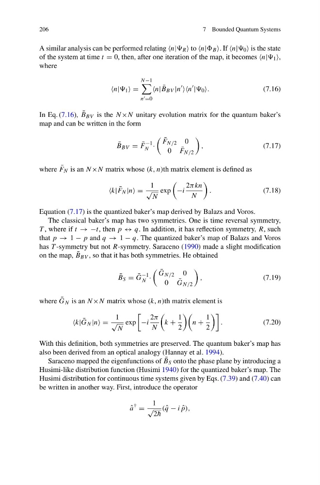
A similar analysis can be performed relating n| R to n| B . If n| 0 is the state
of the system at time t = 0, then, after one iteration of the map, it becomes n| 1 ,
where
n| 1 =
N −1
n =0
n| ¯
B BV |n
n
| 0 .
(7.16)
In Eq. (7.16), ¯
B BV is the N×N unitary evolution matrix for the quantum baker’s
map and can be written in the form
¯
B BV = ¯
F
−1
N ·
¯
F N/2 0
0 ¯
F N/2
,
(7.17)
where ¯
F N is an N×N matrix whose (k, n)th matrix element is defined as
k| ¯
F N |n =
1
√
N
exp
−i
2πkn
N
.
(7.18)
Equation (7.17) is the quantized baker’s map derived by Balazs and Voros.
The classical baker’s map has two symmetries. One is time reversal symmetry,
T , where if t → −t, then p ↔ q. In addition, it has reflection symmetry, R, such
that p → 1 − p and q → 1 − q. The quantized baker’s map of Balazs and Voros
has T -symmetry but not R-symmetry. Saraceno (1990) made a slight modification
on the map, ¯
B BV , so that it has both symmetries. He obtained
¯
B S = ¯
G
−1
N ·
¯
G N/2 0
0 ¯
G N/2
,
(7.19)
where ¯
G N is an N ×N matrix whose (k, n)th matrix element is
k| ¯
G N |n =
1
√
N
exp
−i
2π
N
k +
1
2
n +
1
2
.
(7.20)
With this definition, both symmetries are preserved. The quantum baker’s map has
also been derived from an optical analogy (Hannay et al. 1994).
Saraceno mapped the eigenfunctions of ¯
B S onto the phase plane by introducing a
Husimi-like distribution function (Husimi 1940) for the quantized baker’s map. The
Husimi distribution for continuous time systems given by Eqs. (7.39) and (7.40) can
be written in another way. First, introduce the operator
ˆ
a
†
=
1
√
2 ¯
h
( ˆ
q − i ˆ
p),
7 Bounded Quantum Systems
A similar analysis can be performed relating n| R to n| B . If n| 0 is the state
of the system at time t = 0, then, after one iteration of the map, it becomes n| 1 ,
where
n| 1 =
N −1
n =0
n| ¯
B BV |n
n
| 0 .
(7.16)
In Eq. (7.16), ¯
B BV is the N×N unitary evolution matrix for the quantum baker’s
map and can be written in the form
¯
B BV = ¯
F
−1
N ·
¯
F N/2 0
0 ¯
F N/2
,
(7.17)
where ¯
F N is an N×N matrix whose (k, n)th matrix element is defined as
k| ¯
F N |n =
1
√
N
exp
−i
2πkn
N
.
(7.18)
Equation (7.17) is the quantized baker’s map derived by Balazs and Voros.
The classical baker’s map has two symmetries. One is time reversal symmetry,
T , where if t → −t, then p ↔ q. In addition, it has reflection symmetry, R, such
that p → 1 − p and q → 1 − q. The quantized baker’s map of Balazs and Voros
has T -symmetry but not R-symmetry. Saraceno (1990) made a slight modification
on the map, ¯
B BV , so that it has both symmetries. He obtained
¯
B S = ¯
G
−1
N ·
¯
G N/2 0
0 ¯
G N/2
,
(7.19)
where ¯
G N is an N ×N matrix whose (k, n)th matrix element is
k| ¯
G N |n =
1
√
N
exp
−i
2π
N
k +
1
2
n +
1
2
.
(7.20)
With this definition, both symmetries are preserved. The quantum baker’s map has
also been derived from an optical analogy (Hannay et al. 1994).
Saraceno mapped the eigenfunctions of ¯
B S onto the phase plane by introducing a
Husimi-like distribution function (Husimi 1940) for the quantized baker’s map. The
Husimi distribution for continuous time systems given by Eqs. (7.39) and (7.40) can
be written in another way. First, introduce the operator
ˆ
a
†
=
1
√
2 ¯
h
( ˆ
q − i ˆ
p),