

176
6 Quantum Dynamics and Random Matrix Theory
Information about correlations between eigenvalues is contained in the two-body
cluster function, Y 2 (ξ 1 , ξ 2 ). For a random sequence of eigenvalues, Y 2 (ξ 1 , ξ 2 ) = 0
and it is easy to find the 3 -statistic. We set Y 2 (ξ 1 , ξ 2 ) = 0 in Eqs. (6.88)–(6.90)
and then use Eq. (6.82) to obtain
3
(RAN D)
=
2m
15
=
N
15
.
(6.91)
For a random sequence of eigenvalues, the variance of fluctuations about the mean
grows linearly with the number of levels in the sequence, as one might expect
(Reichl 2016).
In the remainder of this section, we will obtain an explicit expression for the
3 -statistic for the case of the Gaussian orthogonal ensemble. The 3 -statistic is
completely determined by the form of the two-body cluster function, T N (x 1 , x 2 ),
as can be seen from Eqs. (6.86) and (6.87). Therefore, we can use Eq. (6.50)
to find an expression for the 3 -statistic for the Gaussian orthogonal ensemble.
Equation (6.82) and Eqs. (6.88)–(6.90) were obtained assuming that the eigenvalue
sequence has been unfolded and therefore has constant average density. This limit
is obtained for finite eigenvalue sequences whose eigenvalues satisfy the condition
x j
√
2N , and therefore, we will consider this limiting regime. From Eq. (6.77),
the average spacing between eigenvalues is D = π/
√
2N . We can rescale the
eigenvalues x j = Dξ j , and take the limit N→∞ so that ξ j = x j /D is finite.
This is the regime in which we obtain the 3 -statistic for the Gaussian orthogonal
ensemble.
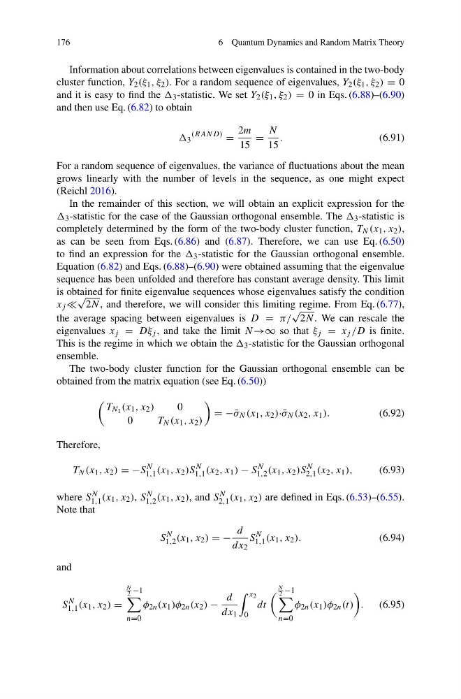
The two-body cluster function for the Gaussian orthogonal ensemble can be
obtained from the matrix equation (see Eq. (6.50))
T N 1 (x 1 , x 2 )
0
0
T N (x 1 , x 2 )
= − ¯
σ N (x 1 , x 2 )· ¯
σ N (x 2 , x 1 ).
(6.92)
Therefore,
T N (x 1 , x 2 ) = −S
N
1,1 (x 1 , x 2 )S
N
1,1 (x 2 , x 1 ) − S
N
1,2 (x 1 , x 2 )S
N
2,1 (x 2 , x 1 ),
(6.93)
where S N
1,1 (x 1 , x 2 ), S N
1,2 (x 1 , x 2 ), and S N
2,1 (x 1 , x 2 ) are defined in Eqs. (6.53)–(6.55).
Note that
S
N
1,2 (x 1 , x 2 ) = −
d
dx 2
S
N
1,1 (x 1 , x 2 ).
(6.94)
and
S
N
1,1 (x 1 , x 2 ) =
N
2 −1
n=0
φ 2n (x 1 )φ 2n (x 2 ) −
d
dx 1
x 2
0
dt
N
2 −1
n=0
φ 2n (x 1 )φ 2n (t)
.
(6.95)
6 Quantum Dynamics and Random Matrix Theory
Information about correlations between eigenvalues is contained in the two-body
cluster function, Y 2 (ξ 1 , ξ 2 ). For a random sequence of eigenvalues, Y 2 (ξ 1 , ξ 2 ) = 0
and it is easy to find the 3 -statistic. We set Y 2 (ξ 1 , ξ 2 ) = 0 in Eqs. (6.88)–(6.90)
and then use Eq. (6.82) to obtain
3
(RAN D)
=
2m
15
=
N
15
.
(6.91)
For a random sequence of eigenvalues, the variance of fluctuations about the mean
grows linearly with the number of levels in the sequence, as one might expect
(Reichl 2016).
In the remainder of this section, we will obtain an explicit expression for the
3 -statistic for the case of the Gaussian orthogonal ensemble. The 3 -statistic is
completely determined by the form of the two-body cluster function, T N (x 1 , x 2 ),
as can be seen from Eqs. (6.86) and (6.87). Therefore, we can use Eq. (6.50)
to find an expression for the 3 -statistic for the Gaussian orthogonal ensemble.
Equation (6.82) and Eqs. (6.88)–(6.90) were obtained assuming that the eigenvalue
sequence has been unfolded and therefore has constant average density. This limit
is obtained for finite eigenvalue sequences whose eigenvalues satisfy the condition
x j
√
2N , and therefore, we will consider this limiting regime. From Eq. (6.77),
the average spacing between eigenvalues is D = π/
√
2N . We can rescale the
eigenvalues x j = Dξ j , and take the limit N→∞ so that ξ j = x j /D is finite.
This is the regime in which we obtain the 3 -statistic for the Gaussian orthogonal
ensemble.
The two-body cluster function for the Gaussian orthogonal ensemble can be
obtained from the matrix equation (see Eq. (6.50))
T N 1 (x 1 , x 2 )
0
0
T N (x 1 , x 2 )
= − ¯
σ N (x 1 , x 2 )· ¯
σ N (x 2 , x 1 ).
(6.92)
Therefore,
T N (x 1 , x 2 ) = −S
N
1,1 (x 1 , x 2 )S
N
1,1 (x 2 , x 1 ) − S
N
1,2 (x 1 , x 2 )S
N
2,1 (x 2 , x 1 ),
(6.93)
where S N
1,1 (x 1 , x 2 ), S N
1,2 (x 1 , x 2 ), and S N
2,1 (x 1 , x 2 ) are defined in Eqs. (6.53)–(6.55).
Note that
S
N
1,2 (x 1 , x 2 ) = −
d
dx 2
S
N
1,1 (x 1 , x 2 ).
(6.94)
and
S
N
1,1 (x 1 , x 2 ) =
N
2 −1
n=0
φ 2n (x 1 )φ 2n (x 2 ) −
d
dx 1
x 2
0
dt
N
2 −1
n=0
φ 2n (x 1 )φ 2n (t)
.
(6.95)