

166
6 Quantum Dynamics and Random Matrix Theory
R N (x 1 , x 2 , x 3 ) = T N (x 1 , x 2 , x 3 ) + T N (x 1 )T N (x 2 , x 3 )
+T N (x 2 )T N (x 1 , x 3 ) + T N (x 3 )T N (x 1 , x 2 ) + T N (x 1 )T N (x 2 )T N (x 3 ),
(6.48)
etc. We can revert the series in Eqs. (6.46)–(6.48) to express the cluster
functions T N (x 1 , x 2 , . . . , x n ) in terms of the reduced joint probability densities
R N (x 1 , x 2 , . . . , x n ).
Explicit expressions for the cluster functions for the Gaussian Orthogonal
Ensemble were obtained in Appendix F. For example,
T N (x 1 ) ¯
1 = ¯
σ N (x 1 , x 1 ),
(6.49)
T N (x 1 , x 2 ) ¯
1 = − ¯
σ N (x 1 , x 2 )· ¯
σ N (x 2 , x 1 ),
(6.50)
and
T N (x 1 , x 2 , x 3 ) ¯
1 = ¯
σ N (x 1 , x 2 )· ¯
σ N (x 2 , x 3 )· ¯
σ N (x 3 , x 1 )
− ¯
σ N (x 1 , x 3 )· ¯
σ N (x 3 , x 2 )· ¯
σ N (x 2 , x 1 ).
(6.51)
Here we let ¯
σ N (i, j ) ≡ ¯
σ N (x i , x j ), where ¯
σ N 1 (i, j ) is the 2×2 matrix
¯
σ N (i, j ) =
S N
1,1 (x i , x j ) S N
1,2 (x i , x j )
S N
2,1 (x i , x j ) S N
1,1 (x j , x i )
(6.52)
and ¯
1 =
1 0
0 1
.
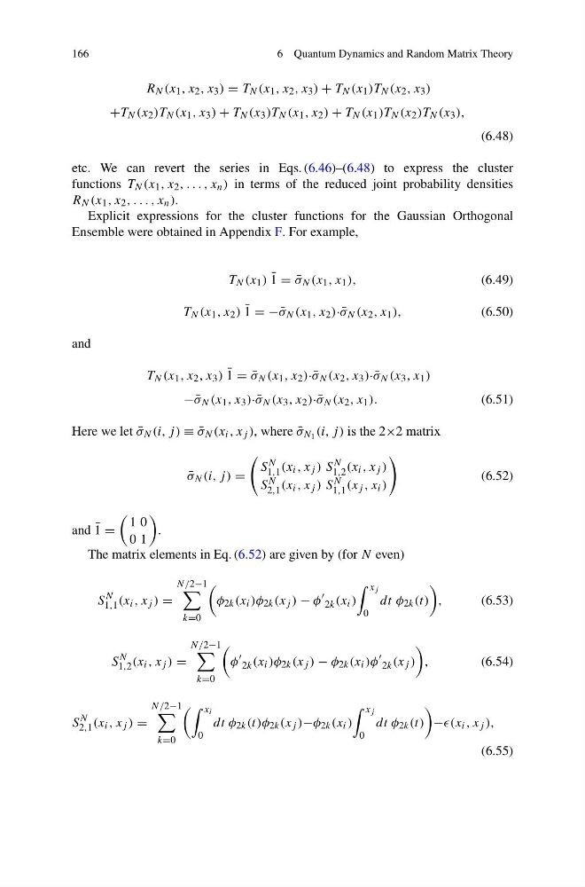
The matrix elements in Eq. (6.52) are given by (for N even)
S
N
1,1 (x i , x j ) =
N/2−1
k=0
φ 2k (x i )φ 2k (x j ) − φ
2k (x i )
x j
0
dt φ 2k (t)
,
(6.53)
S
N
1,2 (x i , x j ) =
N/2−1
k=0
φ
2k (x i )φ 2k (x j ) − φ 2k (x i )φ
2k (x j )
,
(6.54)
S
N
2,1 (x i , x j ) =
N/2−1
k=0
x i
0
dt φ 2k (t)φ 2k (x j )−φ 2k (x i )
x j
0
dt φ 2k (t)
− i , x j ),
(6.55)
6 Quantum Dynamics and Random Matrix Theory
R N (x 1 , x 2 , x 3 ) = T N (x 1 , x 2 , x 3 ) + T N (x 1 )T N (x 2 , x 3 )
+T N (x 2 )T N (x 1 , x 3 ) + T N (x 3 )T N (x 1 , x 2 ) + T N (x 1 )T N (x 2 )T N (x 3 ),
(6.48)
etc. We can revert the series in Eqs. (6.46)–(6.48) to express the cluster
functions T N (x 1 , x 2 , . . . , x n ) in terms of the reduced joint probability densities
R N (x 1 , x 2 , . . . , x n ).
Explicit expressions for the cluster functions for the Gaussian Orthogonal
Ensemble were obtained in Appendix F. For example,
T N (x 1 ) ¯
1 = ¯
σ N (x 1 , x 1 ),
(6.49)
T N (x 1 , x 2 ) ¯
1 = − ¯
σ N (x 1 , x 2 )· ¯
σ N (x 2 , x 1 ),
(6.50)
and
T N (x 1 , x 2 , x 3 ) ¯
1 = ¯
σ N (x 1 , x 2 )· ¯
σ N (x 2 , x 3 )· ¯
σ N (x 3 , x 1 )
− ¯
σ N (x 1 , x 3 )· ¯
σ N (x 3 , x 2 )· ¯
σ N (x 2 , x 1 ).
(6.51)
Here we let ¯
σ N (i, j ) ≡ ¯
σ N (x i , x j ), where ¯
σ N 1 (i, j ) is the 2×2 matrix
¯
σ N (i, j ) =
S N
1,1 (x i , x j ) S N
1,2 (x i , x j )
S N
2,1 (x i , x j ) S N
1,1 (x j , x i )
(6.52)
and ¯
1 =
1 0
0 1
.
The matrix elements in Eq. (6.52) are given by (for N even)
S
N
1,1 (x i , x j ) =
N/2−1
k=0
φ 2k (x i )φ 2k (x j ) − φ
2k (x i )
x j
0
dt φ 2k (t)
,
(6.53)
S
N
1,2 (x i , x j ) =
N/2−1
k=0
φ
2k (x i )φ 2k (x j ) − φ 2k (x i )φ
2k (x j )
,
(6.54)
S
N
2,1 (x i , x j ) =
N/2−1
k=0
x i
0
dt φ 2k (t)φ 2k (x j )−φ 2k (x i )
x j
0
dt φ 2k (t)
− i , x j ),
(6.55)