

108
4 Chaotic Scattering
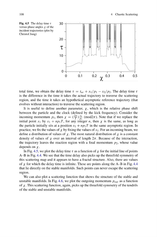
Fig. 4.5 The delay time τ
versus phase angles χ of the
incident trajectories (plot by
Christof Jung)
total time, we obtain the delay time τ = t ac + x 1 /p 1 − x 2 /p 2 . The delay time τ
is the difference in the time it takes the actual trajectory to traverse the scattering
region, and the time it takes an hypothetical asymptotic reference trajectory (that
evolves without interaction) to traverse the scattering region.
It is useful to define another parameter, χ , which is the relative phase shift
between the particle and the clock (defined by the kick frequency). Consider the
incoming momentum p 1 , then χ = (
2π
T )
x 1
p 1
(mod2π ). Note that if we replace the
initial point x 1 by x 1 + np 1 T , for any integer n, then χ is the same, as long as
the particle initially sits at a position x 1 + np 1 T in the same asymptotic region. In
practice, we fix the values of χ by fixing the values of x 1 . For an incoming beam, we
define a distribution of values of χ . The most natural distribution of χ is a constant
density of values of χ over an interval of length 2π . Because of the interaction,
the trajectory leaves the reaction region with a final momentum p 2 , whose value
depends on χ .
In Fig. 4.5, we plot the delay time τ as a function of χ for the initial line of points
A–B in Fig. 4.4. We see that the time delay also picks up the threefold symmetry of
this scattering map and it appears to have a fractal structure. Also, there are values
of χ for which the delay time is infinite. These are points along the A–B in Fig. 4.4
that lie directly on the stable manifolds. Such points can never escape the scattering
region.
We can also plot a scattering function that shows the structure of the stable and
unstable manifolds. In Fig. 4.6, we plot the outgoing momentum p out as a function
of χ . This scattering function, again, picks up the threefold symmetry of the tendrils
of the stable and unstable manifolds.
4 Chaotic Scattering
Fig. 4.5 The delay time τ
versus phase angles χ of the
incident trajectories (plot by
Christof Jung)
total time, we obtain the delay time τ = t ac + x 1 /p 1 − x 2 /p 2 . The delay time τ
is the difference in the time it takes the actual trajectory to traverse the scattering
region, and the time it takes an hypothetical asymptotic reference trajectory (that
evolves without interaction) to traverse the scattering region.
It is useful to define another parameter, χ , which is the relative phase shift
between the particle and the clock (defined by the kick frequency). Consider the
incoming momentum p 1 , then χ = (
2π
T )
x 1
p 1
(mod2π ). Note that if we replace the
initial point x 1 by x 1 + np 1 T , for any integer n, then χ is the same, as long as
the particle initially sits at a position x 1 + np 1 T in the same asymptotic region. In
practice, we fix the values of χ by fixing the values of x 1 . For an incoming beam, we
define a distribution of values of χ . The most natural distribution of χ is a constant
density of values of χ over an interval of length 2π . Because of the interaction,
the trajectory leaves the reaction region with a final momentum p 2 , whose value
depends on χ .
In Fig. 4.5, we plot the delay time τ as a function of χ for the initial line of points
A–B in Fig. 4.4. We see that the time delay also picks up the threefold symmetry of
this scattering map and it appears to have a fractal structure. Also, there are values
of χ for which the delay time is infinite. These are points along the A–B in Fig. 4.4
that lie directly on the stable manifolds. Such points can never escape the scattering
region.
We can also plot a scattering function that shows the structure of the stable and
unstable manifolds. In Fig. 4.6, we plot the outgoing momentum p out as a function
of χ . This scattering function, again, picks up the threefold symmetry of the tendrils
of the stable and unstable manifolds.