

4.2 The Complete Ternary Horseshoe
107
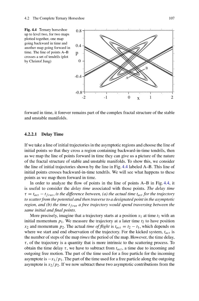
Fig. 4.4 Ternary horseshoe
up to level two, for two maps
plotted together, one map
going backward in time and
another map going forward in
time. The line of points A–B
crosses a set of tendrils (plot
by Christof Jung)
forward in time, it forever remains part of the complex fractal structure of the stable
and unstable manifolds.
4.2.2.1 Delay Time
If we take a line of initial trajectories in the asymptotic regions and choose the line of
initial points so that they cross a region containing backward-in-time tendrils, then
as we map the line of points forward in time they can give us a picture of the nature
of the fractal structure of stable and unstable manifolds. To show this, we consider
the line of initial trajectories shown by the line in Fig. 4.4 labeled A–B. This line of
initial points crosses backward-in-time tendrils. We will see what happens to these
points as we map them forward in time.
In order to analyze the flow of points in the line of points A–B in Fig. 4.4, it
is useful to consider the delay time associated with those points. The delay time
τ = t act − t f ree , is the difference between, (a) the actual time t act for the trajectory
to scatter from the potential and then traverse to a designated point in the asymptotic
region, and (b) the time t f ree a free trajectory would spend traversing between the
same initial and final points.
More precisely, imagine that a trajectory starts at a position x 1 at time t 1 with an
initial momentum p 1 . We measure the trajectory at a later time t 2 to have position
x 2 and momentum p 2 . The actual time of flight is t act = t 2 − t 1 , which depends on
where we start and end observation of the trajectory. For the kicked system, t act is
the number of steps of the map times the period of the map. However, the time delay,
τ , of the trajectory is a quantity that is more intrinsic to the scattering process. To
obtain the time delay τ , we have to subtract from t act , a time due to incoming and
outgoing free motion. The part of the time used for a free particle for the incoming
asymptote is −x 1 /p 1 . The part of the time used for a free particle along the outgoing
asymptote is x 2 /p 2 . If we now subtract these two asymptotic contributions from the
107
Fig. 4.4 Ternary horseshoe
up to level two, for two maps
plotted together, one map
going backward in time and
another map going forward in
time. The line of points A–B
crosses a set of tendrils (plot
by Christof Jung)
forward in time, it forever remains part of the complex fractal structure of the stable
and unstable manifolds.
4.2.2.1 Delay Time
If we take a line of initial trajectories in the asymptotic regions and choose the line of
initial points so that they cross a region containing backward-in-time tendrils, then
as we map the line of points forward in time they can give us a picture of the nature
of the fractal structure of stable and unstable manifolds. To show this, we consider
the line of initial trajectories shown by the line in Fig. 4.4 labeled A–B. This line of
initial points crosses backward-in-time tendrils. We will see what happens to these
points as we map them forward in time.
In order to analyze the flow of points in the line of points A–B in Fig. 4.4, it
is useful to consider the delay time associated with those points. The delay time
τ = t act − t f ree , is the difference between, (a) the actual time t act for the trajectory
to scatter from the potential and then traverse to a designated point in the asymptotic
region, and (b) the time t f ree a free trajectory would spend traversing between the
same initial and final points.
More precisely, imagine that a trajectory starts at a position x 1 at time t 1 with an
initial momentum p 1 . We measure the trajectory at a later time t 2 to have position
x 2 and momentum p 2 . The actual time of flight is t act = t 2 − t 1 , which depends on
where we start and end observation of the trajectory. For the kicked system, t act is
the number of steps of the map times the period of the map. However, the time delay,
τ , of the trajectory is a quantity that is more intrinsic to the scattering process. To
obtain the time delay τ , we have to subtract from t act , a time due to incoming and
outgoing free motion. The part of the time used for a free particle for the incoming
asymptote is −x 1 /p 1 . The part of the time used for a free particle along the outgoing
asymptote is x 2 /p 2 . If we now subtract these two asymptotic contributions from the