

94
3 Area-Preserving Maps
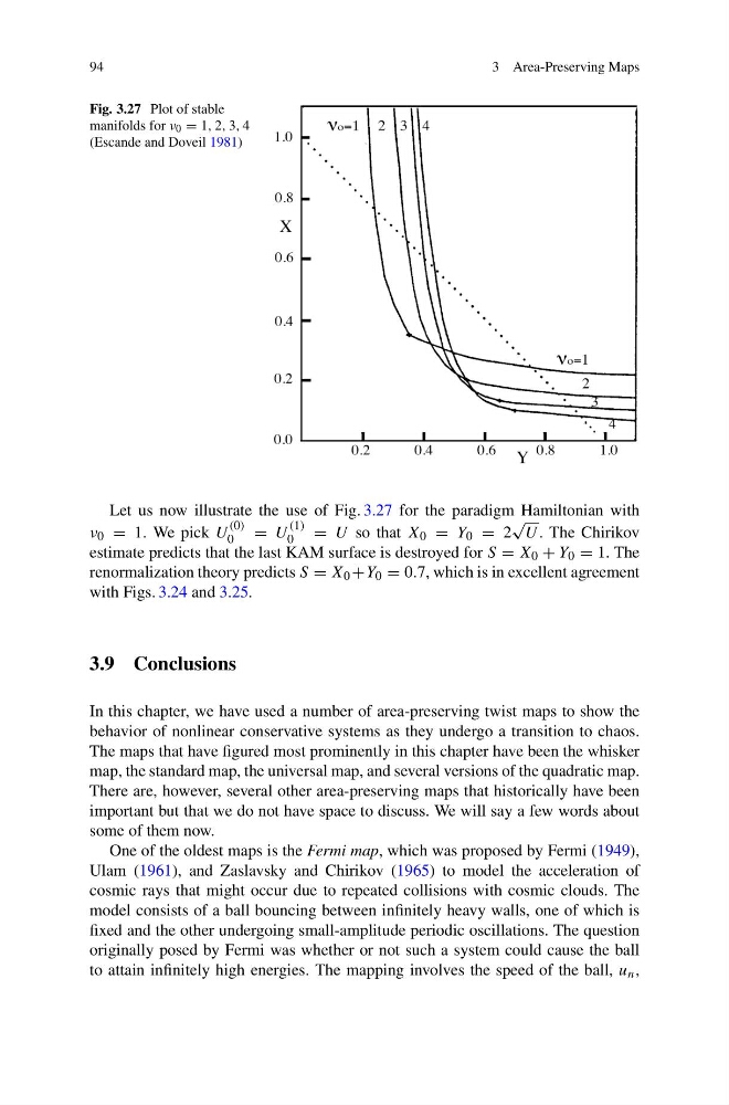
Fig. 3.27 Plot of stable
manifolds for ν 0 = 1, 2, 3, 4
(Escande and Doveil 1981)
Let us now illustrate the use of Fig. 3.27 for the paradigm Hamiltonian with
ν 0 = 1. We pick U
(0)
0
= U
(1)
0
= U so that X 0 = Y 0 = 2
√
U . The Chirikov
estimate predicts that the last KAM surface is destroyed for S = X 0 + Y 0 = 1. The
renormalization theory predicts S = X 0 +Y 0 = 0.7, which is in excellent agreement
with Figs. 3.24 and 3.25.
3.9 Conclusions
In this chapter, we have used a number of area-preserving twist maps to show the
behavior of nonlinear conservative systems as they undergo a transition to chaos.
The maps that have figured most prominently in this chapter have been the whisker
map, the standard map, the universal map, and several versions of the quadratic map.
There are, however, several other area-preserving maps that historically have been
important but that we do not have space to discuss. We will say a few words about
some of them now.
One of the oldest maps is the Fermi map, which was proposed by Fermi (1949),
Ulam (1961), and Zaslavsky and Chirikov (1965) to model the acceleration of
cosmic rays that might occur due to repeated collisions with cosmic clouds. The
model consists of a ball bouncing between infinitely heavy walls, one of which is
fixed and the other undergoing small-amplitude periodic oscillations. The question
originally posed by Fermi was whether or not such a system could cause the ball
to attain infinitely high energies. The mapping involves the speed of the ball, u n ,
3 Area-Preserving Maps
Fig. 3.27 Plot of stable
manifolds for ν 0 = 1, 2, 3, 4
(Escande and Doveil 1981)
Let us now illustrate the use of Fig. 3.27 for the paradigm Hamiltonian with
ν 0 = 1. We pick U
(0)
0
= U
(1)
0
= U so that X 0 = Y 0 = 2
√
U . The Chirikov
estimate predicts that the last KAM surface is destroyed for S = X 0 + Y 0 = 1. The
renormalization theory predicts S = X 0 +Y 0 = 0.7, which is in excellent agreement
with Figs. 3.24 and 3.25.
3.9 Conclusions
In this chapter, we have used a number of area-preserving twist maps to show the
behavior of nonlinear conservative systems as they undergo a transition to chaos.
The maps that have figured most prominently in this chapter have been the whisker
map, the standard map, the universal map, and several versions of the quadratic map.
There are, however, several other area-preserving maps that historically have been
important but that we do not have space to discuss. We will say a few words about
some of them now.
One of the oldest maps is the Fermi map, which was proposed by Fermi (1949),
Ulam (1961), and Zaslavsky and Chirikov (1965) to model the acceleration of
cosmic rays that might occur due to repeated collisions with cosmic clouds. The
model consists of a ball bouncing between infinitely heavy walls, one of which is
fixed and the other undergoing small-amplitude periodic oscillations. The question
originally posed by Fermi was whether or not such a system could cause the ball
to attain infinitely high energies. The mapping involves the speed of the ball, u n ,