

50
D. J. Fernández
3.1 Second-Degree PHA
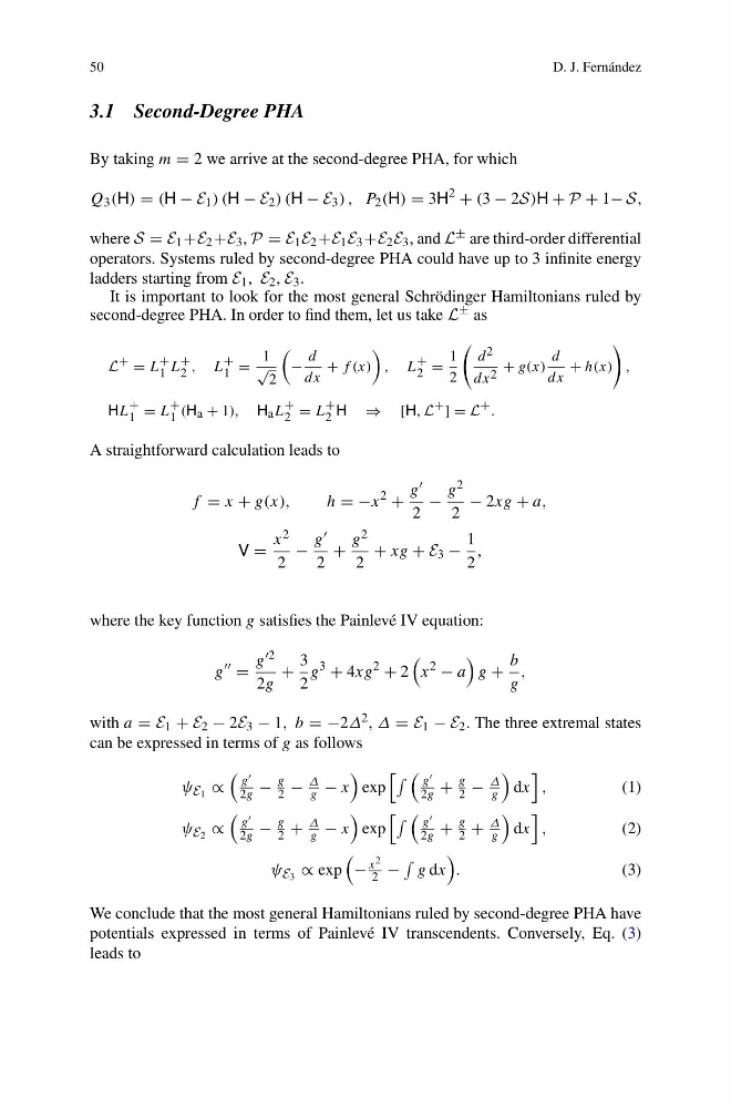
By taking m = 2 we arrive at the second-degree PHA, for which
Q 3 (H) = (H − E 1 ) (H − E 2 ) (H − E 3 ) , P 2 (H) = 3H
2
+ (3 − 2S)H + P + 1− S,
where S = E 1 +E 2 +E 3 , P = E 1 E 2 +E 1 E 3 +E 2 E 3 , and L ± are third-order differential
operators. Systems ruled by second-degree PHA could have up to 3 infinite energy
ladders starting from E 1 , E 2 , E 3 .
It is important to look for the most general Schrödinger Hamiltonians ruled by
second-degree PHA. In order to find them, let us take L ± as
L + = L
+
1 L
+
2 , L
+
1 =
1
√
2
−
d
dx
+ f (x)
, L
+
2 =
1
2
d 2
dx 2 + g(x)
d
dx
+ h(x)
,
HL
+
1 = L
+
1 (H a + 1), H a L
+
2 = L
+
2 H ⇒ [H, L + ] = L + .
A straightforward calculation leads to
f = x + g(x),
h = −x
2
+
g
2
−
g 2
2
− 2xg + a,
V =
x 2
2
−
g
2
+
g 2
2
+ xg + E 3 −
1
2
,
where the key function g satisfies the Painlevé IV equation:
g
=
g
2g
+
3
2
g
3
+ 4xg
2
+ 2
x
2
− a
g +
b
g
,
with a = E 1 + E 2 − 2E 3 − 1, b = −2Δ 2 , Δ = E 1 − E 2 . The three extremal states
can be expressed in terms of g as follows
ψ E 1 ∝
g
2g −
g
2 −
Δ
g − x
exp
g
2g +
g
2 −
Δ
g
dx
,
(1)
ψ E 2 ∝
g
2g −
g
2 +
Δ
g − x
exp
g
2g +
g
2 +
Δ
g
dx
,
(2)
ψ E 3 ∝ exp
−
x 2
2 −
g dx
.
(3)
We conclude that the most general Hamiltonians ruled by second-degree PHA have
potentials expressed in terms of Painlevé IV transcendents. Conversely, Eq. (3)
leads to
D. J. Fernández
3.1 Second-Degree PHA
By taking m = 2 we arrive at the second-degree PHA, for which
Q 3 (H) = (H − E 1 ) (H − E 2 ) (H − E 3 ) , P 2 (H) = 3H
2
+ (3 − 2S)H + P + 1− S,
where S = E 1 +E 2 +E 3 , P = E 1 E 2 +E 1 E 3 +E 2 E 3 , and L ± are third-order differential
operators. Systems ruled by second-degree PHA could have up to 3 infinite energy
ladders starting from E 1 , E 2 , E 3 .
It is important to look for the most general Schrödinger Hamiltonians ruled by
second-degree PHA. In order to find them, let us take L ± as
L + = L
+
1 L
+
2 , L
+
1 =
1
√
2
−
d
dx
+ f (x)
, L
+
2 =
1
2
d 2
dx 2 + g(x)
d
dx
+ h(x)
,
HL
+
1 = L
+
1 (H a + 1), H a L
+
2 = L
+
2 H ⇒ [H, L + ] = L + .
A straightforward calculation leads to
f = x + g(x),
h = −x
2
+
g
2
−
g 2
2
− 2xg + a,
V =
x 2
2
−
g
2
+
g 2
2
+ xg + E 3 −
1
2
,
where the key function g satisfies the Painlevé IV equation:
g
=
g
2g
+
3
2
g
3
+ 4xg
2
+ 2
x
2
− a
g +
b
g
,
with a = E 1 + E 2 − 2E 3 − 1, b = −2Δ 2 , Δ = E 1 − E 2 . The three extremal states
can be expressed in terms of g as follows
ψ E 1 ∝
g
2g −
g
2 −
Δ
g − x
exp
g
2g +
g
2 −
Δ
g
dx
,
(1)
ψ E 2 ∝
g
2g −
g
2 +
Δ
g − x
exp
g
2g +
g
2 +
Δ
g
dx
,
(2)
ψ E 3 ∝ exp
−
x 2
2 −
g dx
.
(3)
We conclude that the most general Hamiltonians ruled by second-degree PHA have
potentials expressed in terms of Painlevé IV transcendents. Conversely, Eq. (3)
leads to