

636
M. Zaimi et al.
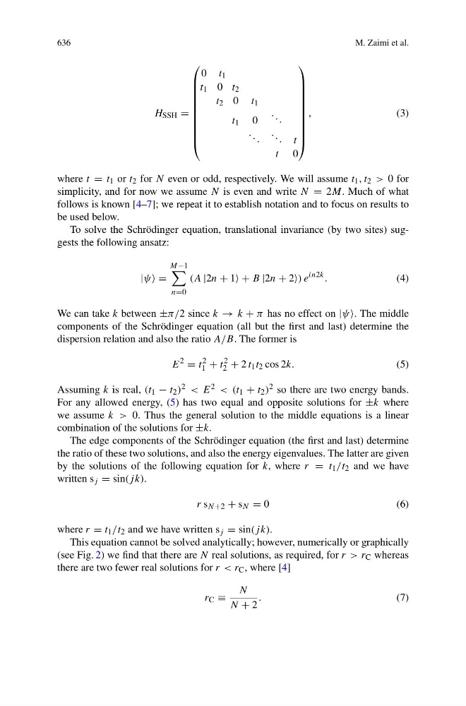
H SSH =
⎛
⎜
⎜
⎜
⎜
⎜
⎜
⎜
⎜
⎜
⎝
0 t 1
t 1 0 t 2
t 2 0 t 1
t 1 0
. . .
. . .
. . . t
t 0
⎞
⎟
⎟
⎟
⎟
⎟
⎟
⎟
⎟
⎟
⎠
,
(3)
where t = t 1 or t 2 for N even or odd, respectively. We will assume t 1 , t 2 > 0 for
simplicity, and for now we assume N is even and write N = 2M. Much of what
follows is known [4–7]; we repeat it to establish notation and to focus on results to
be used below.
To solve the Schrödinger equation, translational invariance (by two sites) suggests the following ansatz:
|ψ =
M−1
n=0
(A |2n + 1 + B |2n + 2) e
in2k .
(4)
We can take k between ±π/2 since k → k + π has no effect on |ψ. The middle
components of the Schrödinger equation (all but the first and last) determine the
dispersion relation and also the ratio A/B. The former is
E
2
= t
2
1 + t
2
2 + 2 t 1 t 2 cos 2k.
(5)
Assuming k is real, (t 1 − t 2 ) 2 < E 2 < (t 1 + t 2 ) 2 so there are two energy bands.
For any allowed energy, (5) has two equal and opposite solutions for ±k where
we assume k > 0. Thus the general solution to the middle equations is a linear
combination of the solutions for ±k.
The edge components of the Schrödinger equation (the first and last) determine
the ratio of these two solutions, and also the energy eigenvalues. The latter are given
by the solutions of the following equation for k, where r = t 1 /t 2 and we have
written s j = sin(jk).
r s N +2 + s N = 0
( 6 )
where r = t 1 /t 2 and we have written s j = sin(jk).
This equation cannot be solved analytically; however, numerically or graphically
(see Fig. 2) we find that there are N real solutions, as required, for r > r C whereas
there are two fewer real solutions for r < r C , where [4]
r C ≡
N
N + 2
.
(7)
M. Zaimi et al.
H SSH =
⎛
⎜
⎜
⎜
⎜
⎜
⎜
⎜
⎜
⎜
⎝
0 t 1
t 1 0 t 2
t 2 0 t 1
t 1 0
. . .
. . .
. . . t
t 0
⎞
⎟
⎟
⎟
⎟
⎟
⎟
⎟
⎟
⎟
⎠
,
(3)
where t = t 1 or t 2 for N even or odd, respectively. We will assume t 1 , t 2 > 0 for
simplicity, and for now we assume N is even and write N = 2M. Much of what
follows is known [4–7]; we repeat it to establish notation and to focus on results to
be used below.
To solve the Schrödinger equation, translational invariance (by two sites) suggests the following ansatz:
|ψ =
M−1
n=0
(A |2n + 1 + B |2n + 2) e
in2k .
(4)
We can take k between ±π/2 since k → k + π has no effect on |ψ. The middle
components of the Schrödinger equation (all but the first and last) determine the
dispersion relation and also the ratio A/B. The former is
E
2
= t
2
1 + t
2
2 + 2 t 1 t 2 cos 2k.
(5)
Assuming k is real, (t 1 − t 2 ) 2 < E 2 < (t 1 + t 2 ) 2 so there are two energy bands.
For any allowed energy, (5) has two equal and opposite solutions for ±k where
we assume k > 0. Thus the general solution to the middle equations is a linear
combination of the solutions for ±k.
The edge components of the Schrödinger equation (the first and last) determine
the ratio of these two solutions, and also the energy eigenvalues. The latter are given
by the solutions of the following equation for k, where r = t 1 /t 2 and we have
written s j = sin(jk).
r s N +2 + s N = 0
( 6 )
where r = t 1 /t 2 and we have written s j = sin(jk).
This equation cannot be solved analytically; however, numerically or graphically
(see Fig. 2) we find that there are N real solutions, as required, for r > r C whereas
there are two fewer real solutions for r < r C , where [4]
r C ≡
N
N + 2
.
(7)