

626
G. Chiribella and Swati
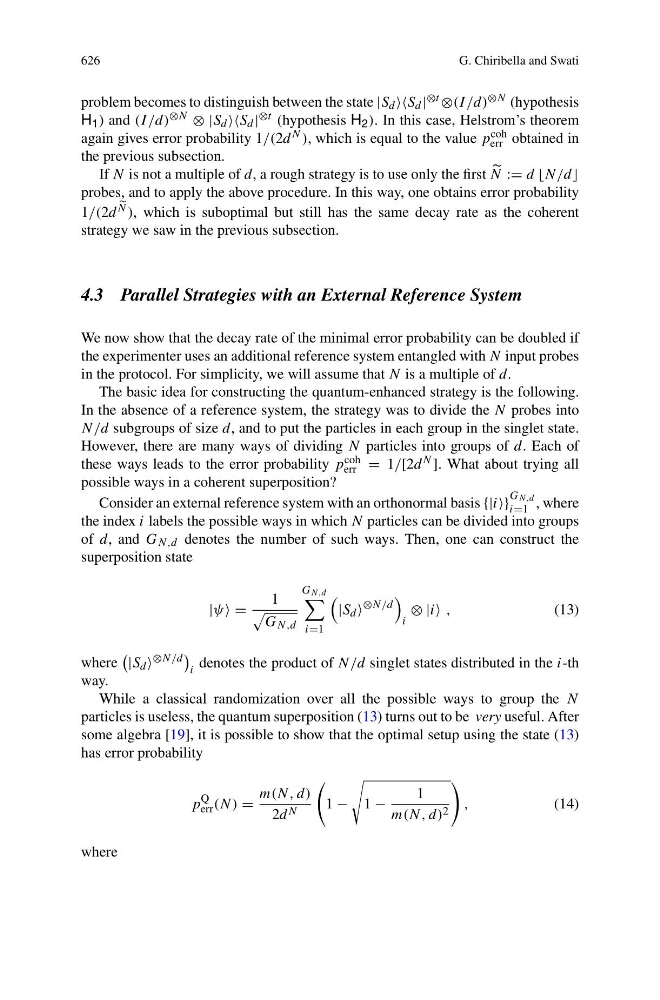
problem becomes to distinguish between the state |S d d | ⊗t ⊗(I /d) ⊗N (hypothesis
H 1 ) and (I /d) ⊗N ⊗ |S d d | ⊗t (hypothesis H 2 ). In this case, Helstrom’s theorem
again gives error probability 1/(2d N ), which is equal to the value p coh
err obtained in
the previous subsection.
If N is not a multiple of d, a rough strategy is to use only the first
N := d N/d
probes, and to apply the above procedure. In this way, one obtains error probability
1/(2d
N ), which is suboptimal but still has the same decay rate as the coherent
strategy we saw in the previous subsection.
4.3 Parallel Strategies with an External Reference System
We now show that the decay rate of the minimal error probability can be doubled if
the experimenter uses an additional reference system entangled with N input probes
in the protocol. For simplicity, we will assume that N is a multiple of d.
The basic idea for constructing the quantum-enhanced strategy is the following.
In the absence of a reference system, the strategy was to divide the N probes into
N/d subgroups of size d, and to put the particles in each group in the singlet state.
However, there are many ways of dividing N particles into groups of d. Each of
these ways leads to the error probability p coh
err = 1/[2d N ]. What about trying all
possible ways in a coherent superposition?
Consider an external reference system with an orthonormal basis {|i}
G N,d
i=1 , where
the index i labels the possible ways in which N particles can be divided into groups
of d, and G N,d denotes the number of such ways. Then, one can construct the
superposition state
|ψ =
1
G N,d
G N,d
i=1
|S d
⊗N/d
i
⊗ |i ,
(13)
where
|S d ⊗N/d
i
denotes the product of N/d singlet states distributed in the i-th
way.
While a classical randomization over all the possible ways to group the N
particles is useless, the quantum superposition (13) turns out to be very useful. After
some algebra [19], it is possible to show that the optimal setup using the state (13)
has error probability
p
Q
err (N) =
m(N, d)
2d N
1 −
1 −
1
m(N, d) 2
,
(14)
where
G. Chiribella and Swati
problem becomes to distinguish between the state |S d d | ⊗t ⊗(I /d) ⊗N (hypothesis
H 1 ) and (I /d) ⊗N ⊗ |S d d | ⊗t (hypothesis H 2 ). In this case, Helstrom’s theorem
again gives error probability 1/(2d N ), which is equal to the value p coh
err obtained in
the previous subsection.
If N is not a multiple of d, a rough strategy is to use only the first
N := d N/d
probes, and to apply the above procedure. In this way, one obtains error probability
1/(2d
N ), which is suboptimal but still has the same decay rate as the coherent
strategy we saw in the previous subsection.
4.3 Parallel Strategies with an External Reference System
We now show that the decay rate of the minimal error probability can be doubled if
the experimenter uses an additional reference system entangled with N input probes
in the protocol. For simplicity, we will assume that N is a multiple of d.
The basic idea for constructing the quantum-enhanced strategy is the following.
In the absence of a reference system, the strategy was to divide the N probes into
N/d subgroups of size d, and to put the particles in each group in the singlet state.
However, there are many ways of dividing N particles into groups of d. Each of
these ways leads to the error probability p coh
err = 1/[2d N ]. What about trying all
possible ways in a coherent superposition?
Consider an external reference system with an orthonormal basis {|i}
G N,d
i=1 , where
the index i labels the possible ways in which N particles can be divided into groups
of d, and G N,d denotes the number of such ways. Then, one can construct the
superposition state
|ψ =
1
G N,d
G N,d
i=1
|S d
⊗N/d
i
⊗ |i ,
(13)
where
|S d ⊗N/d
i
denotes the product of N/d singlet states distributed in the i-th
way.
While a classical randomization over all the possible ways to group the N
particles is useless, the quantum superposition (13) turns out to be very useful. After
some algebra [19], it is possible to show that the optimal setup using the state (13)
has error probability
p
Q
err (N) =
m(N, d)
2d N
1 −
1 −
1
m(N, d) 2
,
(14)
where