

580
D. London
which suggests trying to explain the data by allowing NP to contribute to this decay.
The model-independent starting point is the effective Hamiltonian
H eff = −
αG F
√
2π
V tb V
∗
ts
a=9,10
(C a O a + C
a O
a ) ,
(7)
where O 9(10) = [¯ sγ μ P L b][ ¯
μγ μ (γ 5 )μ], and the primed operators have L → R. The
Wilson coefficients include both SM and NP contributions: C X = C X,SM +C X,NP .
Performing a combined fit to all the data, in the simplest scenarios it is found that
the data can be explained if 1
(i) C
μμ
9,NP
= −1.10 ± 0.16 ,
(ii) C
μμ
9,NP
= −C
μμ
10,NP
= −0.53 ± 0.08 ,
(8)
with a pull of close to 6σ (!). (I note in passing that scenario (ii) involves purely
left-handed NP.)
2.2 b → cτ − ¯
ν
There is another set of observables whose measurements also exhibit discrepancies
with the SM. They involve the decay b → cτ − ¯
ν. This is a ΔQ em = 1 process, and
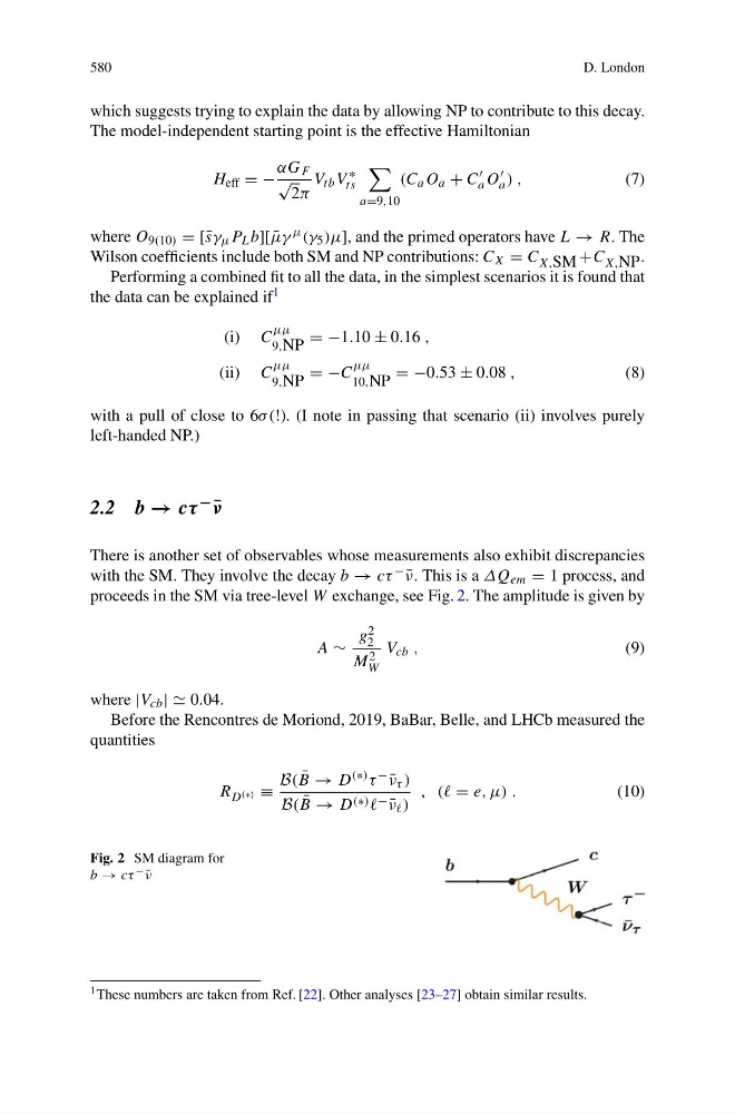
proceeds in the SM via tree-level W exchange, see Fig. 2. The amplitude is given by
A ∼
g 2
2
M 2
W
V cb ,
(9)
where |V cb | | 0.04.
Before the Rencontres de Moriond, 2019, BaBar, Belle, and LHCb measured the
quantities
R D (∗) ≡
B( ¯
B → D (∗) τ − ¯
ν τ )
B( ¯
B → D (∗) − ¯
ν )
, (( = e, μ) .
(10)
Fig. 2 SM diagram for
b → cτ − ¯
ν
1 These numbers are taken from Ref. [22]. Other analyses [23–27] obtain similar results.
D. London
which suggests trying to explain the data by allowing NP to contribute to this decay.
The model-independent starting point is the effective Hamiltonian
H eff = −
αG F
√
2π
V tb V
∗
ts
a=9,10
(C a O a + C
a O
a ) ,
(7)
where O 9(10) = [¯ sγ μ P L b][ ¯
μγ μ (γ 5 )μ], and the primed operators have L → R. The
Wilson coefficients include both SM and NP contributions: C X = C X,SM +C X,NP .
Performing a combined fit to all the data, in the simplest scenarios it is found that
the data can be explained if 1
(i) C
μμ
9,NP
= −1.10 ± 0.16 ,
(ii) C
μμ
9,NP
= −C
μμ
10,NP
= −0.53 ± 0.08 ,
(8)
with a pull of close to 6σ (!). (I note in passing that scenario (ii) involves purely
left-handed NP.)
2.2 b → cτ − ¯
ν
There is another set of observables whose measurements also exhibit discrepancies
with the SM. They involve the decay b → cτ − ¯
ν. This is a ΔQ em = 1 process, and
proceeds in the SM via tree-level W exchange, see Fig. 2. The amplitude is given by
A ∼
g 2
2
M 2
W
V cb ,
(9)
where |V cb | | 0.04.
Before the Rencontres de Moriond, 2019, BaBar, Belle, and LHCb measured the
quantities
R D (∗) ≡
B( ¯
B → D (∗) τ − ¯
ν τ )
B( ¯
B → D (∗) − ¯
ν )
, (( = e, μ) .
(10)
Fig. 2 SM diagram for
b → cτ − ¯
ν
1 These numbers are taken from Ref. [22]. Other analyses [23–27] obtain similar results.