

Electron in Bilayer Graphene with Magnetic Fields Associated with Solvable Potentials
271
-2
-1
1
2
k
1
2
3
4
2 m*
E
h
2
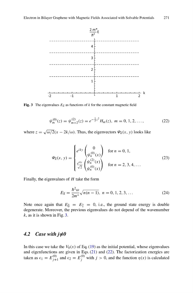
Fig. 3 The eigenvalues E n as functions of k for the constant magnetic field
ψ
(0)
m (z) = ψ
(2)
m+2 (z) = e
−
1
2 z 2 H m (z), m = 0, 1, 2, . . . ,
(22)
where z =
√
ω/2(x − 2k/ω). Thus, the eigenvectors Ψ n (x, y) looks like
Ψ n (x, y) =
⎧
⎪ ⎪ ⎪ ⎪ ⎨
⎪ ⎪ ⎪ ⎪ ⎩
e iky
0
ψ
(0)
n (x)
for n = 0, 1,
e iky
√
2
ψ
(2)
n (x)
ψ
(0)
n (x)
for n = 2, 3, 4, . . .
(23)
Finally, the eigenvalues of H take the form
E n =
¯
h 2 ω
2m ∗
n(n − 1), n = 0, 1, 2, 3, . . .
(24)
Note once again that E 0 = E 1 = 0, i.e., the ground state energy is double
degenerate. Moreover, the previous eigenvalues do not depend of the wavenumber
k, as it is shown in Fig. 3.
4.2 Case with j =0
In this case we take the V 0 (x) of Eq. (19) as the initial potential, whose eigenvalues
and eigenfunctions are given in Eqs. (21) and (22). The factorization energies are
taken as 1 = E
(0)
j +1 and 2 = E
(0)
j with j > 0, and the function η(x) is calculated
271
-2
-1
1
2
k
1
2
3
4
2 m*
E
h
2
Fig. 3 The eigenvalues E n as functions of k for the constant magnetic field
ψ
(0)
m (z) = ψ
(2)
m+2 (z) = e
−
1
2 z 2 H m (z), m = 0, 1, 2, . . . ,
(22)
where z =
√
ω/2(x − 2k/ω). Thus, the eigenvectors Ψ n (x, y) looks like
Ψ n (x, y) =
⎧
⎪ ⎪ ⎪ ⎪ ⎨
⎪ ⎪ ⎪ ⎪ ⎩
e iky
0
ψ
(0)
n (x)
for n = 0, 1,
e iky
√
2
ψ
(2)
n (x)
ψ
(0)
n (x)
for n = 2, 3, 4, . . .
(23)
Finally, the eigenvalues of H take the form
E n =
¯
h 2 ω
2m ∗
n(n − 1), n = 0, 1, 2, 3, . . .
(24)
Note once again that E 0 = E 1 = 0, i.e., the ground state energy is double
degenerate. Moreover, the previous eigenvalues do not depend of the wavenumber
k, as it is shown in Fig. 3.
4.2 Case with j =0
In this case we take the V 0 (x) of Eq. (19) as the initial potential, whose eigenvalues
and eigenfunctions are given in Eqs. (21) and (22). The factorization energies are
taken as 1 = E
(0)
j +1 and 2 = E
(0)
j with j > 0, and the function η(x) is calculated