12
F. Finkel et al.
The procedure outlined above can be applied to the Sutherland model (4) and its
spin version, which yields the original Haldane–Shastry (HS) spin chain [16, 24].
Likewise, from the hyperbolic Calogero–Sutherland model introduced by Inozemtsev [18] one obtains a hyperbolic counterpart of the HS chain usually known as the
Frahm–Inozemtsev (FI) chain [14]. The Hamiltonians of PF, HS, and FI chains can
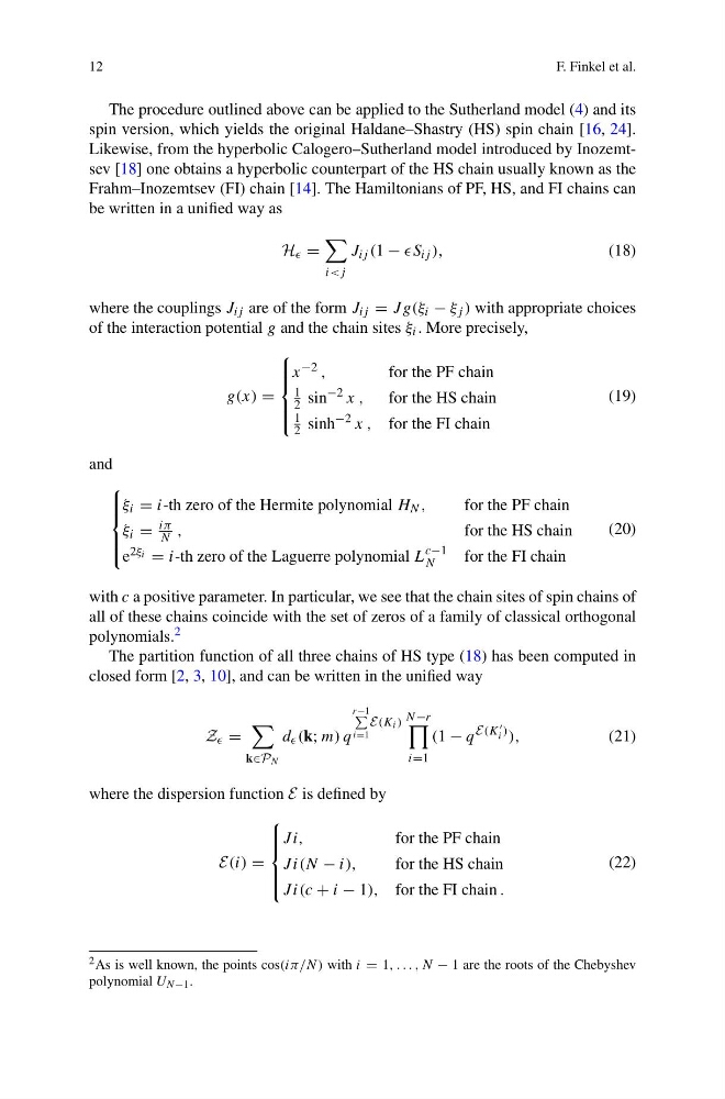
be written in a unified way as
H =
i J ij (1 − S ij ),
(18)
where the couplings J ij are of the form J ij = Jg(ξ i − ξ j ) with appropriate choices
of the interaction potential g and the chain sites ξ i . More precisely,
g(x) =
⎧
⎪ ⎪ ⎨
⎪ ⎪ ⎩
x −2 ,
for the PF chain
1
2 sin
−2 x ,
for the HS chain
1
2 sinh
−2 x , for the FI chain
(19)
and
⎧
⎪ ⎪ ⎨
⎪ ⎪ ⎩
ξ i = i-th zero of the Hermite polynomial H N ,
for the PF chain
ξ i =
iπ
N ,
for the HS chain
e 2ξ i = i-th zero of the Laguerre polynomial L
c−1
N
for the FI chain
(20)
with c a positive parameter. In particular, we see that the chain sites of spin chains of
all of these chains coincide with the set of zeros of a family of classical orthogonal
polynomials. 2
The partition function of all three chains of HS type (18) has been computed in
closed form [2, 3, 10], and can be written in the unified way
Z =
k∈P N
d (k; m) q
r−1
i=1
E(K i ) N −r
i=1
(1 − q
E(K
i ) ),
(21)
where the dispersion function E is defined by
E(i) =
⎧
⎪ ⎪ ⎨
⎪ ⎪ ⎩
J i,
for the PF chain
J i(N − i),
for the HS chain
J i(c + i − 1), for the FI chain .
(22)
2 As is well known, the points cos(iπ/N) with i = 1, . . . , N − 1 are the roots of the Chebyshev
polynomial U N −1 .