

2D Coherent and Squeezed States
261
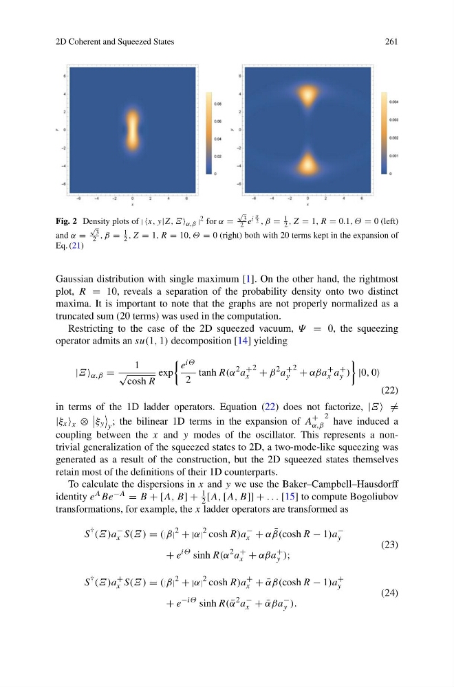
Fig. 2 Density plots of | x, y|Z, Ξ α,β |
2 for α =
√
3
2 e
i
π
2 , β =
1
2 , Z = 1, R = 0.1, Θ = 0 (left)
and α =
√
3
2 , β =
1
2 , Z = 1, R = 10, Θ = 0 (right) both with 20 terms kept in the expansion of
Eq. (21)
Gaussian distribution with single maximum [1]. On the other hand, the rightmost
plot, R = 10, reveals a separation of the probability density onto two distinct
maxima. It is important to note that the graphs are not properly normalized as a
truncated sum (20 terms) was used in the computation.
Restricting to the case of the 2D squeezed vacuum, Ψ = 0, the squeezing
operator admits an su(1, 1) decomposition [14] yielding
|Ξ α,β =
1
√
cosh R
exp
e iΘ
2
tanh R(α
2 a
+
x
2 + β
2 a
+
y
2 + αβa
+
x a
+
y )
|0, 0
(22)
in terms of the 1D ladder operators. Equation (22) does not factorize, |Ξ =
|ξ x x ⊗
ξ y
y
; the bilinear 1D terms in the expansion of A
+
α,β
2 have induced a
coupling between the x and y modes of the oscillator. This represents a nontrivial generalization of the squeezed states to 2D, a two-mode-like squeezing was
generated as a result of the construction, but the 2D squeezed states themselves
retain most of the definitions of their 1D counterparts.
To calculate the dispersions in x and y we use the Baker–Campbell–Hausdorff
identity e A Be −A = B + [A, B] +
1
2 [A, [A, B]] + . . . [15] to compute Bogoliubov
transformations, for example, the x ladder operators are transformed as
S
† (Ξ )a
−
x S(Ξ ) = (|β|
2
+ |α|
2 cosh R)a
−
x + α ¯
β(cosh R − 1)a
−
y
+ e
iΘ sinh R(α
2 a
+
x + αβa
+
y );
(23)
S
† (Ξ )a
+
x S(Ξ ) = (|β|
2
+ |α|
2 cosh R)a
+
x + ¯
αβ(cosh R − 1)a
+
y
+ e
−iΘ sinh R( ¯
α
2 a
−
x + ¯
αβa
−
y ).
(24)
261
Fig. 2 Density plots of | x, y|Z, Ξ α,β |
2 for α =
√
3
2 e
i
π
2 , β =
1
2 , Z = 1, R = 0.1, Θ = 0 (left)
and α =
√
3
2 , β =
1
2 , Z = 1, R = 10, Θ = 0 (right) both with 20 terms kept in the expansion of
Eq. (21)
Gaussian distribution with single maximum [1]. On the other hand, the rightmost
plot, R = 10, reveals a separation of the probability density onto two distinct
maxima. It is important to note that the graphs are not properly normalized as a
truncated sum (20 terms) was used in the computation.
Restricting to the case of the 2D squeezed vacuum, Ψ = 0, the squeezing
operator admits an su(1, 1) decomposition [14] yielding
|Ξ α,β =
1
√
cosh R
exp
e iΘ
2
tanh R(α
2 a
+
x
2 + β
2 a
+
y
2 + αβa
+
x a
+
y )
|0, 0
(22)
in terms of the 1D ladder operators. Equation (22) does not factorize, |Ξ =
|ξ x x ⊗
ξ y
y
; the bilinear 1D terms in the expansion of A
+
α,β
2 have induced a
coupling between the x and y modes of the oscillator. This represents a nontrivial generalization of the squeezed states to 2D, a two-mode-like squeezing was
generated as a result of the construction, but the 2D squeezed states themselves
retain most of the definitions of their 1D counterparts.
To calculate the dispersions in x and y we use the Baker–Campbell–Hausdorff
identity e A Be −A = B + [A, B] +
1
2 [A, [A, B]] + . . . [15] to compute Bogoliubov
transformations, for example, the x ladder operators are transformed as
S
† (Ξ )a
−
x S(Ξ ) = (|β|
2
+ |α|
2 cosh R)a
−
x + α ¯
β(cosh R − 1)a
−
y
+ e
iΘ sinh R(α
2 a
+
x + αβa
+
y );
(23)
S
† (Ξ )a
+
x S(Ξ ) = (|β|
2
+ |α|
2 cosh R)a
+
x + ¯
αβ(cosh R − 1)a
+
y
+ e
−iΘ sinh R( ¯
α
2 a
−
x + ¯
αβa
−
y ).
(24)