

2D Coherent and Squeezed States
259
Table 1 Construction of the
states |ν α,β using the relation
A
+
α,β |ν α,β =
√
ν + 1 |ν + 1 α,β
|ν |n, m
|0 |0, 0
|1 α |1, 0 + β |0, 1
|2 α 2 |2, 0 +
√
2αβ |1, 1 + β 2 |0, 2
. . .
. . .
|ν
n+m=ν
n,m
α n β m
ν
n
|n, m
for α, β ∈ C, I x ⊗ I y = I y ⊗ I x ≡ I and normalization condition |α| 2 + |β| 2 = 1.
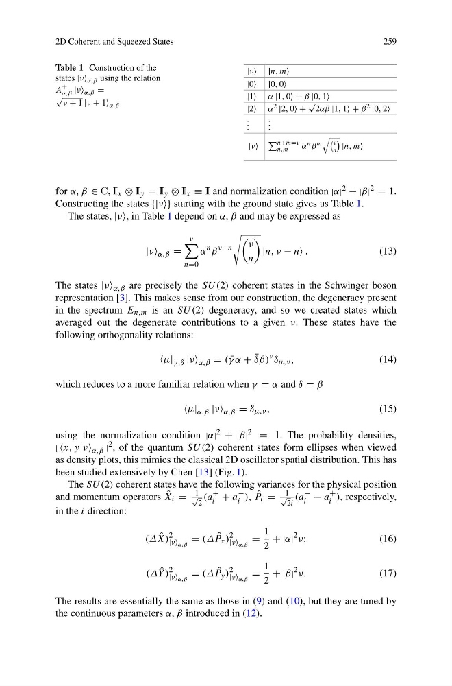
Constructing the states {|ν} starting with the ground state gives us Table 1.
The states, |ν, in Table 1 depend on α, β and may be expressed as
|ν α,β =
ν
n=0
α
n β
ν−n
ν
n
|n, ν − n .
(13)
The states |ν α,β are precisely the SU (2) coherent states in the Schwinger boson
representation [3]. This makes sense from our construction, the degeneracy present
in the spectrum E n,m is an SU (2) degeneracy, and so we created states which
averaged out the degenerate contributions to a given ν. These states have the
following orthogonality relations:
μ| γ,δ |ν α,β = ( ¯
γ α + ¯
δβ)
ν δ μ,ν ,
(14)
which reduces to a more familiar relation when γ = α and δ = β
μ| α,β |ν α,β = δ μ,ν ,
(15)
using the normalization condition |α| 2 + |β| 2 = 1. The probability densities,
| x, y|ν α,β |
2 , of the quantum SU (2) coherent states form ellipses when viewed
as density plots, this mimics the classical 2D oscillator spatial distribution. This has
been studied extensively by Chen [13] (Fig. 1).
The SU (2) coherent states have the following variances for the physical position
and momentum operators ˆ
X i =
1
√
2
(a
+
i + a
−
i ), ˆ
P i =
1
√
2i
(a
−
i − a
+
i ), respectively,
in the i direction:
(Δ ˆ
X)
2
|ν α,β
= (Δ ˆ
P x )
2
|ν α,β
=
1
2
+ |α|
2 ν;
(16)
(Δ ˆ
Y )
2
|ν α,β
= (Δ ˆ
P y )
2
|ν α,β
=
1
2
+ |β|
2 ν.
(17)
The results are essentially the same as those in (9) and (10), but they are tuned by
the continuous parameters α, β introduced in (12).
259
Table 1 Construction of the
states |ν α,β using the relation
A
+
α,β |ν α,β =
√
ν + 1 |ν + 1 α,β
|ν |n, m
|0 |0, 0
|1 α |1, 0 + β |0, 1
|2 α 2 |2, 0 +
√
2αβ |1, 1 + β 2 |0, 2
. . .
. . .
|ν
n+m=ν
n,m
α n β m
ν
n
|n, m
for α, β ∈ C, I x ⊗ I y = I y ⊗ I x ≡ I and normalization condition |α| 2 + |β| 2 = 1.
Constructing the states {|ν} starting with the ground state gives us Table 1.
The states, |ν, in Table 1 depend on α, β and may be expressed as
|ν α,β =
ν
n=0
α
n β
ν−n
ν
n
|n, ν − n .
(13)
The states |ν α,β are precisely the SU (2) coherent states in the Schwinger boson
representation [3]. This makes sense from our construction, the degeneracy present
in the spectrum E n,m is an SU (2) degeneracy, and so we created states which
averaged out the degenerate contributions to a given ν. These states have the
following orthogonality relations:
μ| γ,δ |ν α,β = ( ¯
γ α + ¯
δβ)
ν δ μ,ν ,
(14)
which reduces to a more familiar relation when γ = α and δ = β
μ| α,β |ν α,β = δ μ,ν ,
(15)
using the normalization condition |α| 2 + |β| 2 = 1. The probability densities,
| x, y|ν α,β |
2 , of the quantum SU (2) coherent states form ellipses when viewed
as density plots, this mimics the classical 2D oscillator spatial distribution. This has
been studied extensively by Chen [13] (Fig. 1).
The SU (2) coherent states have the following variances for the physical position
and momentum operators ˆ
X i =
1
√
2
(a
+
i + a
−
i ), ˆ
P i =
1
√
2i
(a
−
i − a
+
i ), respectively,
in the i direction:
(Δ ˆ
X)
2
|ν α,β
= (Δ ˆ
P x )
2
|ν α,β
=
1
2
+ |α|
2 ν;
(16)
(Δ ˆ
Y )
2
|ν α,β
= (Δ ˆ
P y )
2
|ν α,β
=
1
2
+ |β|
2 ν.
(17)
The results are essentially the same as those in (9) and (10), but they are tuned by
the continuous parameters α, β introduced in (12).