

W -Algebras via Lax Type Operators
187
The Hamiltonian reduction (5) still makes sense if we replace associative
algebras with PVAs (respectively, PAs), and we can perform it with A = V(g),
B = V(g >0 ) and I ⊂ B the differential algebra ideal generated by the set (7)
(respectively, A = S(g), B = S(g >0 ), and I ⊂ B the ideal generated by the set (7)).
As a result we get the so-called classical affine W -algebra W aff (g, f ) (respectively,
classical finite W -algebra W aff (g, f )), see [17] for further details.
Unfortunately, a similar construction of a Hamiltonian reduction for vertex
algebras is not known, and the quantum affine W -algebra W aff (g, f ) is constructed
using a cohomological approach [27, 36].
2.4 From the Toy Model to W -Algebras
Let g be a finite-dimensional reductive Lie algebra, and let f ∈ g be a nilpotent
element. By the Jacobson–Morozov Theorem it can be embedded in an sl 2 -triple
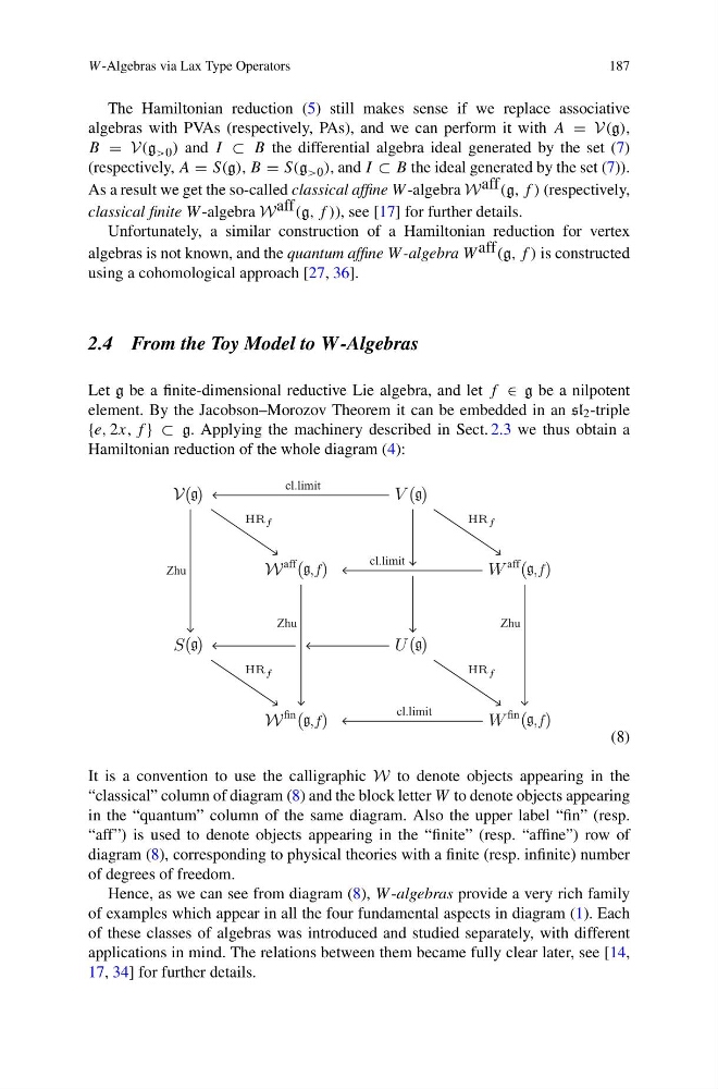
{e, 2x, f } ⊂ g. Applying the machinery described in Sect. 2.3 we thus obtain a
Hamiltonian reduction of the whole diagram (4):
V
Zhu
HR f
V
cl.limit
HR f
W
aff
Zhu
W
aff
cl.limit
Zhu
S
HR f
U
HR f
W
fin
W
fin
cl.limit
( )
( )
( )
( )
,f)
(
,f)
(
,f)
(
,f)
(
(8)
It is a convention to use the calligraphic W to denote objects appearing in the
“classical” column of diagram (8) and the block letter W to denote objects appearing
in the “quantum” column of the same diagram. Also the upper label “fin” (resp.
“aff”) is used to denote objects appearing in the “finite” (resp. “affine”) row of
diagram (8), corresponding to physical theories with a finite (resp. infinite) number
of degrees of freedom.
Hence, as we can see from diagram (8), W -algebras provide a very rich family
of examples which appear in all the four fundamental aspects in diagram (1). Each
of these classes of algebras was introduced and studied separately, with different
applications in mind. The relations between them became fully clear later, see [14,
17, 34] for further details.
187
The Hamiltonian reduction (5) still makes sense if we replace associative
algebras with PVAs (respectively, PAs), and we can perform it with A = V(g),
B = V(g >0 ) and I ⊂ B the differential algebra ideal generated by the set (7)
(respectively, A = S(g), B = S(g >0 ), and I ⊂ B the ideal generated by the set (7)).
As a result we get the so-called classical affine W -algebra W aff (g, f ) (respectively,
classical finite W -algebra W aff (g, f )), see [17] for further details.
Unfortunately, a similar construction of a Hamiltonian reduction for vertex
algebras is not known, and the quantum affine W -algebra W aff (g, f ) is constructed
using a cohomological approach [27, 36].
2.4 From the Toy Model to W -Algebras
Let g be a finite-dimensional reductive Lie algebra, and let f ∈ g be a nilpotent
element. By the Jacobson–Morozov Theorem it can be embedded in an sl 2 -triple
{e, 2x, f } ⊂ g. Applying the machinery described in Sect. 2.3 we thus obtain a
Hamiltonian reduction of the whole diagram (4):
V
Zhu
HR f
V
cl.limit
HR f
W
aff
Zhu
W
aff
cl.limit
Zhu
S
HR f
U
HR f
W
fin
W
fin
cl.limit
( )
( )
( )
( )
,f)
(
,f)
(
,f)
(
,f)
(
(8)
It is a convention to use the calligraphic W to denote objects appearing in the
“classical” column of diagram (8) and the block letter W to denote objects appearing
in the “quantum” column of the same diagram. Also the upper label “fin” (resp.
“aff”) is used to denote objects appearing in the “finite” (resp. “affine”) row of
diagram (8), corresponding to physical theories with a finite (resp. infinite) number
of degrees of freedom.
Hence, as we can see from diagram (8), W -algebras provide a very rich family
of examples which appear in all the four fundamental aspects in diagram (1). Each
of these classes of algebras was introduced and studied separately, with different
applications in mind. The relations between them became fully clear later, see [14,
17, 34] for further details.