

Zernike System from Free Motion on 3-Sphere
173
Φ
I
J,m 1 ,m 2
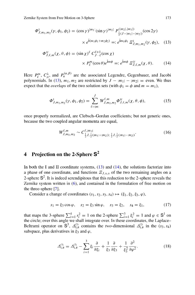
(γ , φ 1 , φ 2 ) = (cos γ )
|m 1 | (sin γ )
|m 2 | P
(|m 2 |,|m 1 |)
1
2 (J −|m 1 |−|m 2 |)
(cos 2γ )
× e i(m 1 φ 1 +m 2 φ 2 ) =: e im 1 φ 1 Ξ
I
J,m 1 ,m 2
(γ , φ 2 ), (13)
Φ
II
J,,,m (χ, θ, φ) = (sin χ)
C
J − (cos χ)
× P
m
(cos θ)e imφ =: e imφ Ξ
II
J,,,m (χ , θ ).
(14)
Here P m
, C λ
μ , and P
(α,β)
n
are the associated Legendre, Gegenbauer, and Jacobi
polynomials. In (13), m 1 , m 2 are restricted by J − |m 1 | − |m 2 | = even. We thus
expect that the overlaps of the two solution sets (with φ 1 = φ and m = m 1 ),
Φ
I
J,m 1 ,m 2
(γ , φ 1 , φ 2 ) =
J
W
,m
J,m 1 ,m 2
Φ
II
J,,,m (χ, θ, φ),
(15)
once properly normalized, are Clebsch–Gordan coefficients; but not generic ones,
because the two coupled angular momenta are equal,
W
,m
J,m 1 ,m 2
∼ C
1 |
1
2 J,
1
2 (|m 1 |+|m 2 |);
1
2 J,
1
2 (|m 1 |−|m 2 |)
.
(16)
4 Projection on the 2-Sphere S
2
In both the I and II coordinate systems, (13) and (14), the solutions factorize into
a phase of one coordinate, and functions Ξ J,◦,◦ of the two remaining angles on a
2-sphere S
2 . It is indeed serendipitous that this reduction to the 2-sphere reveals the
Zernike system written in (6), and contained in the formulation of free motion on
the three-sphere [7].
Consider a change of coordinates (s 1 , s 2 , s 3 , s 4 ) → (ξ 1 , ξ 2 , ξ 3 , ϕ),
s 1 = ξ 3 cos ϕ, s 2 = ξ 3 sin ϕ, s 3 = ξ 2 , s 4 = ξ 1 ,
(17)
that maps the 3-sphere
4
i=1 s 2
i = 1 on the 2-sphere
3
i=1 ξ 2
i = 1 and ϕ ∈ S
1 on
the circle; over this angle we shall integrate over. In these coordinates, the Laplace–
Beltrami operator on S
3 , Δ
(3)
LB contains the two-dimensional Δ
(2)
LB in the (s 3 , s 4 )
subspace, plus derivatives in ξ 3 and ϕ,
Δ
(3)
LB = Δ
(2)
LB −
3
i=1
ξ i
∂
∂ξ i
+
1
ξ 3
∂
∂ξ 3
+
1
ξ 2
3
∂ 2
∂ϕ 2 .
(18)
173
Φ
I
J,m 1 ,m 2
(γ , φ 1 , φ 2 ) = (cos γ )
|m 1 | (sin γ )
|m 2 | P
(|m 2 |,|m 1 |)
1
2 (J −|m 1 |−|m 2 |)
(cos 2γ )
× e i(m 1 φ 1 +m 2 φ 2 ) =: e im 1 φ 1 Ξ
I
J,m 1 ,m 2
(γ , φ 2 ), (13)
Φ
II
J,,,m (χ, θ, φ) = (sin χ)
C
J − (cos χ)
× P
m
(cos θ)e imφ =: e imφ Ξ
II
J,,,m (χ , θ ).
(14)
Here P m
, C λ
μ , and P
(α,β)
n
are the associated Legendre, Gegenbauer, and Jacobi
polynomials. In (13), m 1 , m 2 are restricted by J − |m 1 | − |m 2 | = even. We thus
expect that the overlaps of the two solution sets (with φ 1 = φ and m = m 1 ),
Φ
I
J,m 1 ,m 2
(γ , φ 1 , φ 2 ) =
J
W
,m
J,m 1 ,m 2
Φ
II
J,,,m (χ, θ, φ),
(15)
once properly normalized, are Clebsch–Gordan coefficients; but not generic ones,
because the two coupled angular momenta are equal,
W
,m
J,m 1 ,m 2
∼ C
1 |
1
2 J,
1
2 (|m 1 |+|m 2 |);
1
2 J,
1
2 (|m 1 |−|m 2 |)
.
(16)
4 Projection on the 2-Sphere S
2
In both the I and II coordinate systems, (13) and (14), the solutions factorize into
a phase of one coordinate, and functions Ξ J,◦,◦ of the two remaining angles on a
2-sphere S
2 . It is indeed serendipitous that this reduction to the 2-sphere reveals the
Zernike system written in (6), and contained in the formulation of free motion on
the three-sphere [7].
Consider a change of coordinates (s 1 , s 2 , s 3 , s 4 ) → (ξ 1 , ξ 2 , ξ 3 , ϕ),
s 1 = ξ 3 cos ϕ, s 2 = ξ 3 sin ϕ, s 3 = ξ 2 , s 4 = ξ 1 ,
(17)
that maps the 3-sphere
4
i=1 s 2
i = 1 on the 2-sphere
3
i=1 ξ 2
i = 1 and ϕ ∈ S
1 on
the circle; over this angle we shall integrate over. In these coordinates, the Laplace–
Beltrami operator on S
3 , Δ
(3)
LB contains the two-dimensional Δ
(2)
LB in the (s 3 , s 4 )
subspace, plus derivatives in ξ 3 and ϕ,
Δ
(3)
LB = Δ
(2)
LB −
3
i=1
ξ i
∂
∂ξ i
+
1
ξ 3
∂
∂ξ 3
+
1
ξ 2
3
∂ 2
∂ϕ 2 .
(18)