

158
J. Benson and F. Valiquette
Our computations will closely follow the exposition found in [1]. In this paper, we
will not be able to recall and explain all the results used from [1], and therefore
recommend that the reader reviews [1] for a more detailed exposition.
The main result of this note is that the curvature invariant of a discrete curve
in 2-dimensional Cayley–Klein geometries evolves, under a certain arc-length
preserving flow, according to the integrable differential-difference equation [5],
∂κ n
∂t
= (1 +
2
n+1 )(κ n+1 − κ n−1 ),
where the value of ∈ {−1, 0, 1} is related to the geometry of the Cayley–Klein
plane.
2 Cayley–Klein Planes
Let 1 , , 2 ∈ {−1, 0, 1}, and consider the 3-dimensional Cayley–Klein Lie algebra
so 1 ,, 2 (3) spanned by three vectors P 1 , P 2 , J 12 , with nonzero commutators
[J 12 , P 1 ] = P 2 ,
[J 12 , P 2 ] = − 2 P 1 ,
[P 1 , P 2 ] = 1 J 12 .
Exponentiating so 1 ,, 2 (3) yields the special orthogonal Cayley–Klein group
SO 1 ,, 2 (3) with 1-parameter subgroups
H 1 = {e
εP 1 : ε ∈ R},
H 2 = {e
εP 2 : ε ∈ R},
H 12 = {e
εJ 12 : ε ∈ R}.
Definition 1 The two-dimensional Cayley–Klein planes are defined as the homogeneous spaces
S
2
[ 1 ],, 2
:= SO 1 ,, 2 (3)/H 12 .
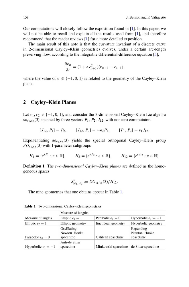
The nine geometries that one obtains appear in Table 1.
Table 1 Two-dimensional Cayley–Klein geometries
Measure of lengths
Measure of angles
Elliptic 1 = 1
Parabolic 1 = 0
Hyperbolic 1 = −1
Elliptic 2 = 1
Elliptic geometry
Euclidean geometry
Hyperbolic geometry
Parabolic 2 = 0
Oscillating
Newton–Hooke
spacetime
Galilean spacetime
Expanding
Newton–Hooke
spacetime
Hyperbolic 2 = −1
Anti-de Sitter
spacetime
Minkowski spacetime de Sitter spacetime
J. Benson and F. Valiquette
Our computations will closely follow the exposition found in [1]. In this paper, we
will not be able to recall and explain all the results used from [1], and therefore
recommend that the reader reviews [1] for a more detailed exposition.
The main result of this note is that the curvature invariant of a discrete curve
in 2-dimensional Cayley–Klein geometries evolves, under a certain arc-length
preserving flow, according to the integrable differential-difference equation [5],
∂κ n
∂t
= (1 +
2
n+1 )(κ n+1 − κ n−1 ),
where the value of ∈ {−1, 0, 1} is related to the geometry of the Cayley–Klein
plane.
2 Cayley–Klein Planes
Let 1 , , 2 ∈ {−1, 0, 1}, and consider the 3-dimensional Cayley–Klein Lie algebra
so 1 ,, 2 (3) spanned by three vectors P 1 , P 2 , J 12 , with nonzero commutators
[J 12 , P 1 ] = P 2 ,
[J 12 , P 2 ] = − 2 P 1 ,
[P 1 , P 2 ] = 1 J 12 .
Exponentiating so 1 ,, 2 (3) yields the special orthogonal Cayley–Klein group
SO 1 ,, 2 (3) with 1-parameter subgroups
H 1 = {e
εP 1 : ε ∈ R},
H 2 = {e
εP 2 : ε ∈ R},
H 12 = {e
εJ 12 : ε ∈ R}.
Definition 1 The two-dimensional Cayley–Klein planes are defined as the homogeneous spaces
S
2
[ 1 ],, 2
:= SO 1 ,, 2 (3)/H 12 .
The nine geometries that one obtains appear in Table 1.
Table 1 Two-dimensional Cayley–Klein geometries
Measure of lengths
Measure of angles
Elliptic 1 = 1
Parabolic 1 = 0
Hyperbolic 1 = −1
Elliptic 2 = 1
Elliptic geometry
Euclidean geometry
Hyperbolic geometry
Parabolic 2 = 0
Oscillating
Newton–Hooke
spacetime
Galilean spacetime
Expanding
Newton–Hooke
spacetime
Hyperbolic 2 = −1
Anti-de Sitter
spacetime
Minkowski spacetime de Sitter spacetime