

Conditional Discretization of PDEs
155
+ h
2 u n+1,m x
2
nm ) − u n,m+1 u n+1,m u nm x nm (x nm + h)
×
h
2
+ k
x nm − hk
− 2hku n,m+1 u
3
nm (x nm + h)
× (hu n+1,m − x nm − h) + ku n,m+1 u
2
n+1,m x
2
nm (hu n+1,m + x nm + h)
−1
.
The existence of this conditional symmetry allows, as in the continuous case,
to simplify the equation—reducing the number of variables in the continuous case
and reducing the number of indices in the discrete case. In this case we can assume
that u nm depends only on the first index (that is, u n,m+1 = u nm ). The difference
equation (13) becomes
u n =
(x n−2 + h)
x
2
n−2 − h(3x n−2 − h)u n−1 − h
2
u
2
n−2
− x n−2
x
2
n−2 − h
2
u n−1 u n−2 − 2h(x n−2 + h)(h(u n−1 − 1) − x n−2 )u
3
n−2
+ x
2
n−2 (h(u n−1 + 1) + x n−2 )u
2
n−1
−1 x
2
n−2 (x n−2 + 2h)u
3
n−1 .
(14)
Equation (2) has the exact conditionally invariant solution (9) depending only on
x. It turns out that in this case, the discrete function and lattice:
u n =
x n
x n − c
, x n+1 = x n + h
(15)
are an exact solution of the difference equation (14) for any constant c and any step
h. The proof is obtained by a direct substitution of (15) into (14). This implies that
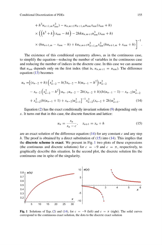
the discrete scheme is exact. We present in Fig. 1 two plots of these expressions
(the continuous and discrete solutions) for c = −9 and c = π , respectively, to
graphically describe this situation. In the second plot, the discrete solution fits the
continuous one in spite of the singularity.
x
u(x)
5
10
15
20
25
30
0.2
0.3
0.4
0.5
0.6
0.7
0.8
u(x)
x
2
3
4
5
6
-10
-5
5
10
Fig. 1 Solutions of Eqs. (2) and (14), for c = −9 (left) and c = π (right). The solid curves
correspond to the continuous exact solution, the dots to the discrete exact solution
155
+ h
2 u n+1,m x
2
nm ) − u n,m+1 u n+1,m u nm x nm (x nm + h)
×
h
2
+ k
x nm − hk
− 2hku n,m+1 u
3
nm (x nm + h)
× (hu n+1,m − x nm − h) + ku n,m+1 u
2
n+1,m x
2
nm (hu n+1,m + x nm + h)
−1
.
The existence of this conditional symmetry allows, as in the continuous case,
to simplify the equation—reducing the number of variables in the continuous case
and reducing the number of indices in the discrete case. In this case we can assume
that u nm depends only on the first index (that is, u n,m+1 = u nm ). The difference
equation (13) becomes
u n =
(x n−2 + h)
x
2
n−2 − h(3x n−2 − h)u n−1 − h
2
u
2
n−2
− x n−2
x
2
n−2 − h
2
u n−1 u n−2 − 2h(x n−2 + h)(h(u n−1 − 1) − x n−2 )u
3
n−2
+ x
2
n−2 (h(u n−1 + 1) + x n−2 )u
2
n−1
−1 x
2
n−2 (x n−2 + 2h)u
3
n−1 .
(14)
Equation (2) has the exact conditionally invariant solution (9) depending only on
x. It turns out that in this case, the discrete function and lattice:
u n =
x n
x n − c
, x n+1 = x n + h
(15)
are an exact solution of the difference equation (14) for any constant c and any step
h. The proof is obtained by a direct substitution of (15) into (14). This implies that
the discrete scheme is exact. We present in Fig. 1 two plots of these expressions
(the continuous and discrete solutions) for c = −9 and c = π , respectively, to
graphically describe this situation. In the second plot, the discrete solution fits the
continuous one in spite of the singularity.
x
u(x)
5
10
15
20
25
30
0.2
0.3
0.4
0.5
0.6
0.7
0.8
u(x)
x
2
3
4
5
6
-10
-5
5
10
Fig. 1 Solutions of Eqs. (2) and (14), for c = −9 (left) and c = π (right). The solid curves
correspond to the continuous exact solution, the dots to the discrete exact solution