

Conditional Discretization of PDEs
153
u =
x
x − c
.
(9)
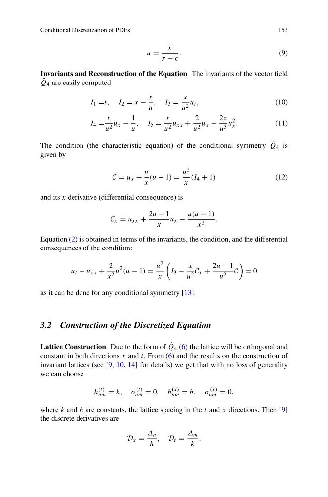
Invariants and Reconstruction of the Equation The invariants of the vector field
ˆ
Q 4 are easily computed
I 1 =t, I 2 = x −
x
u
, I 3 =
x
u 2 u t ,
(10)
I 4 =
x
u 2 u x −
1
u
, I 5 =
x
u 2 u xx +
2
u 2 u x −
2x
u 3 u
2
x .
(11)
The condition (the characteristic equation) of the conditional symmetry ˆ
Q 4 is
given by
C = u x +
u
x
(u − 1) =
u 2
x
(I 4 + 1)
(12)
and its x derivative (differential consequence) is
C x = u xx +
2u − 1
x
u x −
u(u − 1)
x 2 .
Equation (2) is obtained in terms of the invariants, the condition, and the differential
consequences of the condition:
u t − u xx +
2
x 2 u
2 (u − 1) =
u 2
x
I 3 −
x
u 2 C x +
2u − 1
u 2 C
= 0
as it can be done for any conditional symmetry [13].
3.2 Construction of the Discretized Equation
Lattice Construction Due to the form of ˆ
Q 4 (6) the lattice will be orthogonal and
constant in both directions x and t. From (6) and the results on the construction of
invariant lattices (see [9, 10, 14] for details) we get that with no loss of generality
we can choose
h
(t)
nm = k, σ
(t)
nm = 0, h
(x)
nm = h, σ
(x)
nm = 0,
where k and h are constants, the lattice spacing in the t and x directions. Then [9]
the discrete derivatives are
D x =
Δ n
h
, D t =
Δ m
k
.
153
u =
x
x − c
.
(9)
Invariants and Reconstruction of the Equation The invariants of the vector field
ˆ
Q 4 are easily computed
I 1 =t, I 2 = x −
x
u
, I 3 =
x
u 2 u t ,
(10)
I 4 =
x
u 2 u x −
1
u
, I 5 =
x
u 2 u xx +
2
u 2 u x −
2x
u 3 u
2
x .
(11)
The condition (the characteristic equation) of the conditional symmetry ˆ
Q 4 is
given by
C = u x +
u
x
(u − 1) =
u 2
x
(I 4 + 1)
(12)
and its x derivative (differential consequence) is
C x = u xx +
2u − 1
x
u x −
u(u − 1)
x 2 .
Equation (2) is obtained in terms of the invariants, the condition, and the differential
consequences of the condition:
u t − u xx +
2
x 2 u
2 (u − 1) =
u 2
x
I 3 −
x
u 2 C x +
2u − 1
u 2 C
= 0
as it can be done for any conditional symmetry [13].
3.2 Construction of the Discretized Equation
Lattice Construction Due to the form of ˆ
Q 4 (6) the lattice will be orthogonal and
constant in both directions x and t. From (6) and the results on the construction of
invariant lattices (see [9, 10, 14] for details) we get that with no loss of generality
we can choose
h
(t)
nm = k, σ
(t)
nm = 0, h
(x)
nm = h, σ
(x)
nm = 0,
where k and h are constants, the lattice spacing in the t and x directions. Then [9]
the discrete derivatives are
D x =
Δ n
h
, D t =
Δ m
k
.