

116
B. K. Berntson et al.
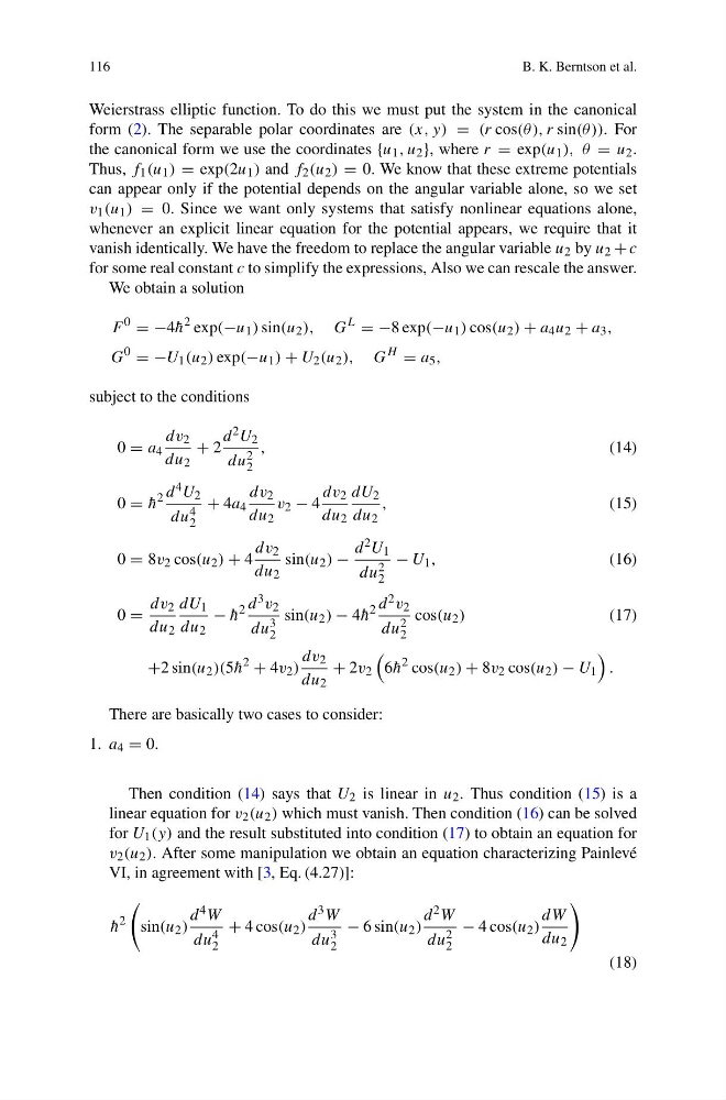
Weierstrass elliptic function. To do this we must put the system in the canonical
form (2). The separable polar coordinates are (x, y) = (r cos(θ ), r sin(θ )). For
the canonical form we use the coordinates {u 1 , u 2 }, where r = exp(u 1 ), θ = u 2 .
Thus, f 1 (u 1 ) = exp(2u 1 ) and f 2 (u 2 ) = 0. We know that these extreme potentials
can appear only if the potential depends on the angular variable alone, so we set
v 1 (u 1 ) = 0. Since we want only systems that satisfy nonlinear equations alone,
whenever an explicit linear equation for the potential appears, we require that it
vanish identically. We have the freedom to replace the angular variable u 2 by u 2 + c
for some real constant c to simplify the expressions, Also we can rescale the answer.
We obtain a solution
F
0
= −4 ¯
h
2 exp(−u 1 ) sin(u 2 ), G
L
= −8 exp(−u 1 ) cos(u 2 ) + a 4 u 2 + a 3 ,
G
0
= −U 1 (u 2 ) exp(−u 1 ) + U 2 (u 2 ), G
H
= a 5 ,
subject to the conditions
0 = a 4
dv 2
du 2
+ 2
d 2 U 2
du 2
2
,
(14)
0 = ¯
h
2 d 4 U 2
du 4
2
+ 4a 4
dv 2
du 2
v 2 − 4
dv 2
du 2
dU 2
du 2
,
(15)
0 = 8v 2 cos(u 2 ) + 4
dv 2
du 2
sin(u 2 ) −
d 2 U 1
du 2
2
− U 1 ,
(16)
0 =
dv 2
du 2
dU 1
du 2
− ¯
h
2 d 3 v 2
du 3
2
sin(u 2 ) − 4 ¯
h
2 d 2 v 2
du 2
2
cos(u 2 )
(17)
+2 sin(u 2 )(5 ¯
h
2
+ 4v 2 )
dv 2
du 2
+ 2v 2
6 ¯
h
2 cos(u 2 ) + 8v 2 cos(u 2 ) − U 1
.
There are basically two cases to consider:
1. a 4 = 0.
Then condition (14) says that U 2 is linear in u 2 . Thus condition (15) is a
linear equation for v 2 (u 2 ) which must vanish. Then condition (16) can be solved
for U 1 (y) and the result substituted into condition (17) to obtain an equation for
v 2 (u 2 ). After some manipulation we obtain an equation characterizing Painlevé
VI, in agreement with [3, Eq. (4.27)]:
¯
h
2
sin(u 2 )
d 4 W
du 4
2
+ 4 cos(u 2 )
d 3 W
du 3
2
− 6 sin(u 2 )
d 2 W
du 2
2
− 4 cos(u 2 )
dW
du 2
(18)
B. K. Berntson et al.
Weierstrass elliptic function. To do this we must put the system in the canonical
form (2). The separable polar coordinates are (x, y) = (r cos(θ ), r sin(θ )). For
the canonical form we use the coordinates {u 1 , u 2 }, where r = exp(u 1 ), θ = u 2 .
Thus, f 1 (u 1 ) = exp(2u 1 ) and f 2 (u 2 ) = 0. We know that these extreme potentials
can appear only if the potential depends on the angular variable alone, so we set
v 1 (u 1 ) = 0. Since we want only systems that satisfy nonlinear equations alone,
whenever an explicit linear equation for the potential appears, we require that it
vanish identically. We have the freedom to replace the angular variable u 2 by u 2 + c
for some real constant c to simplify the expressions, Also we can rescale the answer.
We obtain a solution
F
0
= −4 ¯
h
2 exp(−u 1 ) sin(u 2 ), G
L
= −8 exp(−u 1 ) cos(u 2 ) + a 4 u 2 + a 3 ,
G
0
= −U 1 (u 2 ) exp(−u 1 ) + U 2 (u 2 ), G
H
= a 5 ,
subject to the conditions
0 = a 4
dv 2
du 2
+ 2
d 2 U 2
du 2
2
,
(14)
0 = ¯
h
2 d 4 U 2
du 4
2
+ 4a 4
dv 2
du 2
v 2 − 4
dv 2
du 2
dU 2
du 2
,
(15)
0 = 8v 2 cos(u 2 ) + 4
dv 2
du 2
sin(u 2 ) −
d 2 U 1
du 2
2
− U 1 ,
(16)
0 =
dv 2
du 2
dU 1
du 2
− ¯
h
2 d 3 v 2
du 3
2
sin(u 2 ) − 4 ¯
h
2 d 2 v 2
du 2
2
cos(u 2 )
(17)
+2 sin(u 2 )(5 ¯
h
2
+ 4v 2 )
dv 2
du 2
+ 2v 2
6 ¯
h
2 cos(u 2 ) + 8v 2 cos(u 2 ) − U 1
.
There are basically two cases to consider:
1. a 4 = 0.
Then condition (14) says that U 2 is linear in u 2 . Thus condition (15) is a
linear equation for v 2 (u 2 ) which must vanish. Then condition (16) can be solved
for U 1 (y) and the result substituted into condition (17) to obtain an equation for
v 2 (u 2 ). After some manipulation we obtain an equation characterizing Painlevé
VI, in agreement with [3, Eq. (4.27)]:
¯
h
2
sin(u 2 )
d 4 W
du 4
2
+ 4 cos(u 2 )
d 3 W
du 3
2
− 6 sin(u 2 )
d 2 W
du 2
2
− 4 cos(u 2 )
dW
du 2
(18)