

106
A. Lattanzi
This solution expressed as a recursive series is a proof that the causality (and the
light-cone structure) is not violated by the nonlocality of the Hamiltonian. Each
solution term, ψ n , is determined by recursion on the values assumed previously
by ψ n−1 , till the evolution of the equation has been completely described. Mathematically, the recursive solution (16) allows to find approximations when the exact
solution is not yet known and it is a common procedure to use it to evaluate the
evolution equations with memory terms. In fact the properties of memory and
causality induce a description by means of recursive equations and read-out maps
involving input state and output variables.
In this work, the term “memory” referred to the kernel of the convolution risks
to be too exotic since the convoluted variable is ξ , i.e. the dimensionless variable
related with the space. The recursive solution of the Salpeter equation given by (18)
allows an interesting comparison with the numerical solution and the solution
defined via closed-analytical expression.
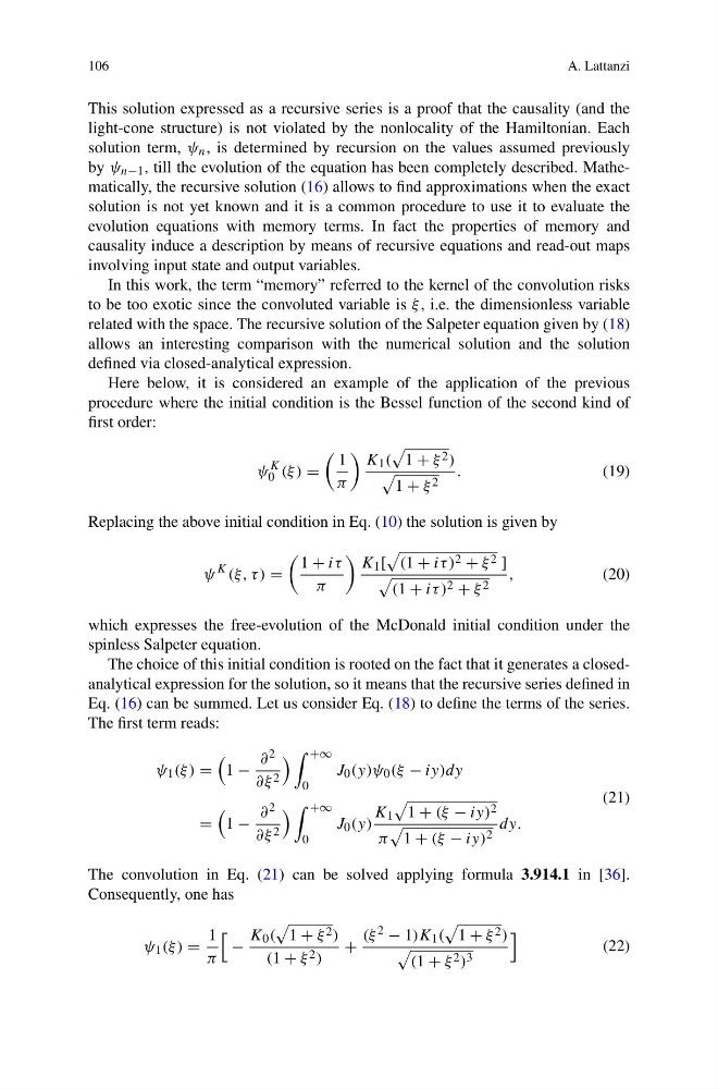
Here below, it is considered an example of the application of the previous
procedure where the initial condition is the Bessel function of the second kind of
first order:
ψ
K
0 (ξ ) =
1
π
K 1 (
1 + ξ 2 )
1 + ξ 2
.
(19)
Replacing the above initial condition in Eq. (10) the solution is given by
ψ
K (ξ, τ ) =
1 + iτ
π
K 1 [
(1 + iτ ) 2 + ξ 2 ]
(1 + iτ ) 2 + ξ 2
,
(20)
which expresses the free-evolution of the McDonald initial condition under the
spinless Salpeter equation.
The choice of this initial condition is rooted on the fact that it generates a closedanalytical expression for the solution, so it means that the recursive series defined in
Eq. (16) can be summed. Let us consider Eq. (18) to define the terms of the series.
The first term reads:
ψ 1 (ξ ) =
1 −
∂ 2
∂ξ 2
+∞
0
J 0 (y)ψ 0 (ξ − iy)dy
=
1 −
∂ 2
∂ξ 2
+∞
0
J 0 (y)
K 1
1 + (ξ − iy) 2
π
1 + (ξ − iy) 2
dy.
(21)
The convolution in Eq. (21) can be solved applying formula 3.914.1 in [36].
Consequently, one has
ψ 1 (ξ ) =
1
π
−
K 0 (
1 + ξ 2 )
(1 + ξ 2 )
+
(ξ 2 − 1)K 1 (
1 + ξ 2 )
(1 + ξ 2 ) 3
(22)
A. Lattanzi
This solution expressed as a recursive series is a proof that the causality (and the
light-cone structure) is not violated by the nonlocality of the Hamiltonian. Each
solution term, ψ n , is determined by recursion on the values assumed previously
by ψ n−1 , till the evolution of the equation has been completely described. Mathematically, the recursive solution (16) allows to find approximations when the exact
solution is not yet known and it is a common procedure to use it to evaluate the
evolution equations with memory terms. In fact the properties of memory and
causality induce a description by means of recursive equations and read-out maps
involving input state and output variables.
In this work, the term “memory” referred to the kernel of the convolution risks
to be too exotic since the convoluted variable is ξ , i.e. the dimensionless variable
related with the space. The recursive solution of the Salpeter equation given by (18)
allows an interesting comparison with the numerical solution and the solution
defined via closed-analytical expression.
Here below, it is considered an example of the application of the previous
procedure where the initial condition is the Bessel function of the second kind of
first order:
ψ
K
0 (ξ ) =
1
π
K 1 (
1 + ξ 2 )
1 + ξ 2
.
(19)
Replacing the above initial condition in Eq. (10) the solution is given by
ψ
K (ξ, τ ) =
1 + iτ
π
K 1 [
(1 + iτ ) 2 + ξ 2 ]
(1 + iτ ) 2 + ξ 2
,
(20)
which expresses the free-evolution of the McDonald initial condition under the
spinless Salpeter equation.
The choice of this initial condition is rooted on the fact that it generates a closedanalytical expression for the solution, so it means that the recursive series defined in
Eq. (16) can be summed. Let us consider Eq. (18) to define the terms of the series.
The first term reads:
ψ 1 (ξ ) =
1 −
∂ 2
∂ξ 2
+∞
0
J 0 (y)ψ 0 (ξ − iy)dy
=
1 −
∂ 2
∂ξ 2
+∞
0
J 0 (y)
K 1
1 + (ξ − iy) 2
π
1 + (ξ − iy) 2
dy.
(21)
The convolution in Eq. (21) can be solved applying formula 3.914.1 in [36].
Consequently, one has
ψ 1 (ξ ) =
1
π
−
K 0 (
1 + ξ 2 )
(1 + ξ 2 )
+
(ξ 2 − 1)K 1 (
1 + ξ 2 )
(1 + ξ 2 ) 3
(22)