

Ellipsometry Techniques and Its Advanced Applications …
577
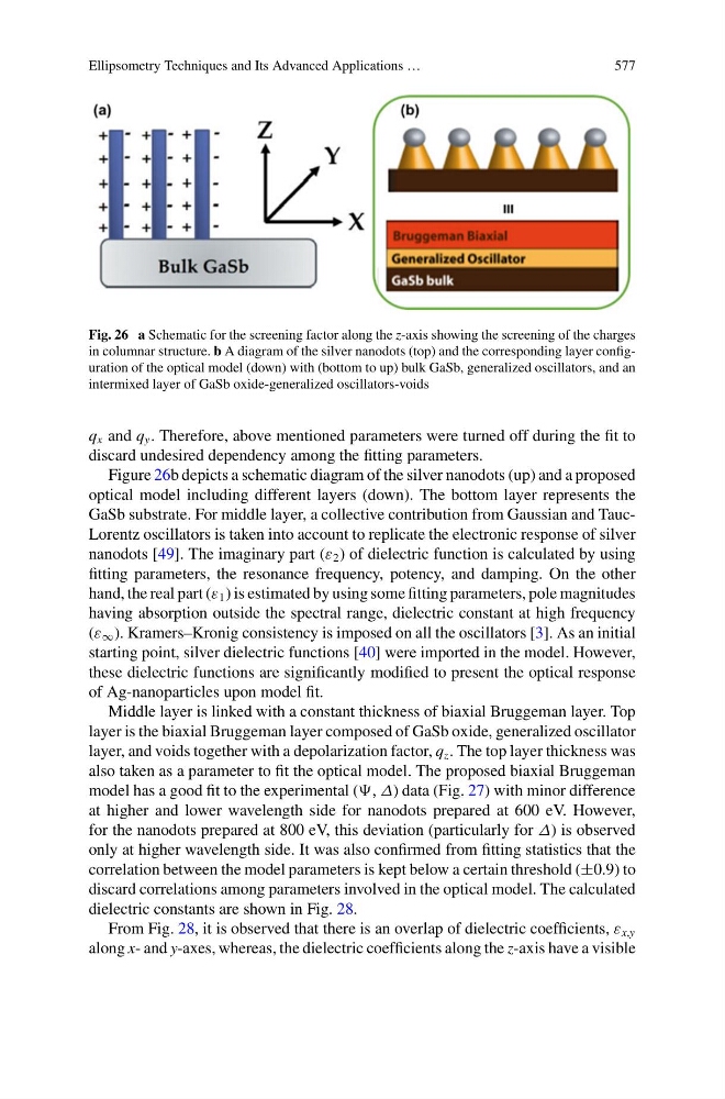
Fig. 26 a Schematic for the screening factor along the z-axis showing the screening of the charges
in columnar structure. b A diagram of the silver nanodots (top) and the corresponding layer configuration of the optical model (down) with (bottom to up) bulk GaSb, generalized oscillators, and an
intermixed layer of GaSb oxide-generalized oscillators-voids
q x and q y . Therefore, above mentioned parameters were turned off during the fit to
discard undesired dependency among the fitting parameters.
Figure 26b depicts a schematic diagram of the silver nanodots (up) and a proposed
optical model including different layers (down). The bottom layer represents the
GaSb substrate. For middle layer, a collective contribution from Gaussian and TaucLorentz oscillators is taken into account to replicate the electronic response of silver
nanodots [49]. The imaginary part (ε 2 ) of dielectric function is calculated by using
fitting parameters, the resonance frequency, potency, and damping. On the other
hand, the real part (ε 1 ) is estimated by using some fitting parameters, pole magnitudes
having absorption outside the spectral range, dielectric constant at high frequency
(ε ∞ ). Kramers–Kronig consistency is imposed on all the oscillators [3]. As an initial
starting point, silver dielectric functions [40] were imported in the model. However,
these dielectric functions are significantly modified to present the optical response
of Ag-nanoparticles upon model fit.
Middle layer is linked with a constant thickness of biaxial Bruggeman layer. Top
layer is the biaxial Bruggeman layer composed of GaSb oxide, generalized oscillator
layer, and voids together with a depolarization factor, q z . The top layer thickness was
also taken as a parameter to fit the optical model. The proposed biaxial Bruggeman
model has a good fit to the experimental (, Δ) data (Fig. 27) with minor difference
at higher and lower wavelength side for nanodots prepared at 600 eV. However,
for the nanodots prepared at 800 eV, this deviation (particularly for Δ) is observed
only at higher wavelength side. It was also confirmed from fitting statistics that the
correlation between the model parameters is kept below a certain threshold (±0.9) to
discard correlations among parameters involved in the optical model. The calculated
dielectric constants are shown in Fig. 28.
From Fig. 28, it is observed that there is an overlap of dielectric coefficients, ε x,y
along x- and y-axes, whereas, the dielectric coefficients along the z-axis have a visible
577
Fig. 26 a Schematic for the screening factor along the z-axis showing the screening of the charges
in columnar structure. b A diagram of the silver nanodots (top) and the corresponding layer configuration of the optical model (down) with (bottom to up) bulk GaSb, generalized oscillators, and an
intermixed layer of GaSb oxide-generalized oscillators-voids
q x and q y . Therefore, above mentioned parameters were turned off during the fit to
discard undesired dependency among the fitting parameters.
Figure 26b depicts a schematic diagram of the silver nanodots (up) and a proposed
optical model including different layers (down). The bottom layer represents the
GaSb substrate. For middle layer, a collective contribution from Gaussian and TaucLorentz oscillators is taken into account to replicate the electronic response of silver
nanodots [49]. The imaginary part (ε 2 ) of dielectric function is calculated by using
fitting parameters, the resonance frequency, potency, and damping. On the other
hand, the real part (ε 1 ) is estimated by using some fitting parameters, pole magnitudes
having absorption outside the spectral range, dielectric constant at high frequency
(ε ∞ ). Kramers–Kronig consistency is imposed on all the oscillators [3]. As an initial
starting point, silver dielectric functions [40] were imported in the model. However,
these dielectric functions are significantly modified to present the optical response
of Ag-nanoparticles upon model fit.
Middle layer is linked with a constant thickness of biaxial Bruggeman layer. Top
layer is the biaxial Bruggeman layer composed of GaSb oxide, generalized oscillator
layer, and voids together with a depolarization factor, q z . The top layer thickness was
also taken as a parameter to fit the optical model. The proposed biaxial Bruggeman
model has a good fit to the experimental (, Δ) data (Fig. 27) with minor difference
at higher and lower wavelength side for nanodots prepared at 600 eV. However,
for the nanodots prepared at 800 eV, this deviation (particularly for Δ) is observed
only at higher wavelength side. It was also confirmed from fitting statistics that the
correlation between the model parameters is kept below a certain threshold (±0.9) to
discard correlations among parameters involved in the optical model. The calculated
dielectric constants are shown in Fig. 28.
From Fig. 28, it is observed that there is an overlap of dielectric coefficients, ε x,y
along x- and y-axes, whereas, the dielectric coefficients along the z-axis have a visible