

Fluorescence Spectrometry
455
and
P =
I − I ⊥
I + I ⊥
(24)
The measured fluorescence anisotropy and polarization are commonly decreased
by the rotational diffusion which occurs during the excitation process in which the
emission dipole of a fluorophore is displaced. But, the influence of rotational diffusion
can be decreased if the fluorophore is bound to a macromolecule. In the case of
spherical fluorophores, the anisotropy decay is a single exponent having a single
rotational correlation time and can be given as: r (t) = r o exp(−t/τ r ); where r o is the
initial anisotropy (anisotropy at time t= 0 or anisotropy observed in the absence of
any depolarizing processes) and τ r is the rotational correlation time. The relationship
between the steady-state anisotropy (r), initial anisotropy (r o ), rotational correlation
time (τ r ) and fluorescence lifetime (τ f ) is given by the Perrin equation:
r o
r
= 1 +
τ f
τ r
(25)
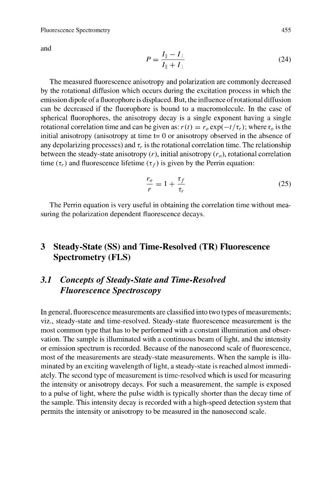
The Perrin equation is very useful in obtaining the correlation time without measuring the polarization dependent fluorescence decays.
3 Steady-State (SS) and Time-Resolved (TR) Fluorescence
Spectrometry (FLS)
3.1 Concepts of Steady-State and Time-Resolved
Fluorescence Spectroscopy
In general, fluorescence measurements are classified into two types of measurements;
viz., steady-state and time-resolved. Steady-state fluorescence measurement is the
most common type that has to be performed with a constant illumination and observation. The sample is illuminated with a continuous beam of light, and the intensity
or emission spectrum is recorded. Because of the nanosecond scale of fluorescence,
most of the measurements are steady-state measurements. When the sample is illuminated by an exciting wavelength of light, a steady-state is reached almost immediately. The second type of measurement is time-resolved which is used for measuring
the intensity or anisotropy decays. For such a measurement, the sample is exposed
to a pulse of light, where the pulse width is typically shorter than the decay time of
the sample. This intensity decay is recorded with a high-speed detection system that
permits the intensity or anisotropy to be measured in the nanosecond scale.
455
and
P =
I − I ⊥
I + I ⊥
(24)
The measured fluorescence anisotropy and polarization are commonly decreased
by the rotational diffusion which occurs during the excitation process in which the
emission dipole of a fluorophore is displaced. But, the influence of rotational diffusion
can be decreased if the fluorophore is bound to a macromolecule. In the case of
spherical fluorophores, the anisotropy decay is a single exponent having a single
rotational correlation time and can be given as: r (t) = r o exp(−t/τ r ); where r o is the
initial anisotropy (anisotropy at time t= 0 or anisotropy observed in the absence of
any depolarizing processes) and τ r is the rotational correlation time. The relationship
between the steady-state anisotropy (r), initial anisotropy (r o ), rotational correlation
time (τ r ) and fluorescence lifetime (τ f ) is given by the Perrin equation:
r o
r
= 1 +
τ f
τ r
(25)
The Perrin equation is very useful in obtaining the correlation time without measuring the polarization dependent fluorescence decays.
3 Steady-State (SS) and Time-Resolved (TR) Fluorescence
Spectrometry (FLS)
3.1 Concepts of Steady-State and Time-Resolved
Fluorescence Spectroscopy
In general, fluorescence measurements are classified into two types of measurements;
viz., steady-state and time-resolved. Steady-state fluorescence measurement is the
most common type that has to be performed with a constant illumination and observation. The sample is illuminated with a continuous beam of light, and the intensity
or emission spectrum is recorded. Because of the nanosecond scale of fluorescence,
most of the measurements are steady-state measurements. When the sample is illuminated by an exciting wavelength of light, a steady-state is reached almost immediately. The second type of measurement is time-resolved which is used for measuring
the intensity or anisotropy decays. For such a measurement, the sample is exposed
to a pulse of light, where the pulse width is typically shorter than the decay time of
the sample. This intensity decay is recorded with a high-speed detection system that
permits the intensity or anisotropy to be measured in the nanosecond scale.