

and Nöllert 1993). In fact, the presence of the tree frog does not seem to be related
to pond size but rather to the amount of terrestrial habitat surrounding the pond
(Vos and Stumpel 1996). Although the aquatic habitat is essential for reproduction,
the species spends most of its time in terrestrial habitats. In agricultural environments, the species often prefers edge habitats like ponds located on river banks,
ditches, fields and forest edges (Pellet et al. 2004).
The seasonal migrations between this terrestrial habitat and the breeding pond
range from 250 to 1000 m (Stumpel 1993). These dispersal events are very
important in the tree frog’s life cycle. Juveniles disperse from the breeding pond
into the surrounding landscape to access other ponds. Despite the fidelity of the tree
frog to its breeding ground, some adults may disperse and change ponds (Fog
1993). Observed dispersal distances are generally less than 2000 m but may reach
up to 4000 m (Vos and Stumpel 1996).
Landscape Data
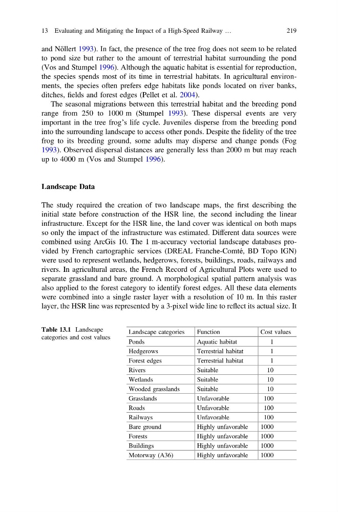
The study required the creation of two landscape maps, the first describing the
initial state before construction of the HSR line, the second including the linear
infrastructure. Except for the HSR line, the land cover was identical on both maps
so only the impact of the infrastructure was estimated. Different data sources were
combined using ArcGis 10. The 1 m-accuracy vectorial landscape databases provided by French cartographic services (DREAL Franche-Comté, BD Topo IGN)
were used to represent wetlands, hedgerows, forests, buildings, roads, railways and
rivers. In agricultural areas, the French Record of Agricultural Plots were used to
separate grassland and bare ground. A morphological spatial pattern analysis was
also applied to the forest category to identify forest edges. All these data elements
were combined into a single raster layer with a resolution of 10 m. In this raster
layer, the HSR line was represented by a 3-pixel wide line to reflect its actual size. It
Table 13.1 Landscape
categories and cost values
Landscape categories
Function
Cost values
Ponds
Aquatic habitat
1
Hedgerows
Terrestrial habitat
1
Forest edges
Terrestrial habitat
1
Rivers
Suitable
10
Wetlands
Suitable
10
Wooded grasslands
Suitable
10
Grasslands
Unfavorable
100
Roads
Unfavorable
100
Railways
Unfavorable
100
Bare ground
Highly unfavorable
1000
Forests
Highly unfavorable
1000
Buildings
Highly unfavorable
1000
Motorway (A36)
Highly unfavorable
1000
13 Evaluating and Mitigating the Impact of a High-Speed Railway …
219
to pond size but rather to the amount of terrestrial habitat surrounding the pond
(Vos and Stumpel 1996). Although the aquatic habitat is essential for reproduction,
the species spends most of its time in terrestrial habitats. In agricultural environments, the species often prefers edge habitats like ponds located on river banks,
ditches, fields and forest edges (Pellet et al. 2004).
The seasonal migrations between this terrestrial habitat and the breeding pond
range from 250 to 1000 m (Stumpel 1993). These dispersal events are very
important in the tree frog’s life cycle. Juveniles disperse from the breeding pond
into the surrounding landscape to access other ponds. Despite the fidelity of the tree
frog to its breeding ground, some adults may disperse and change ponds (Fog
1993). Observed dispersal distances are generally less than 2000 m but may reach
up to 4000 m (Vos and Stumpel 1996).
Landscape Data
The study required the creation of two landscape maps, the first describing the
initial state before construction of the HSR line, the second including the linear
infrastructure. Except for the HSR line, the land cover was identical on both maps
so only the impact of the infrastructure was estimated. Different data sources were
combined using ArcGis 10. The 1 m-accuracy vectorial landscape databases provided by French cartographic services (DREAL Franche-Comté, BD Topo IGN)
were used to represent wetlands, hedgerows, forests, buildings, roads, railways and
rivers. In agricultural areas, the French Record of Agricultural Plots were used to
separate grassland and bare ground. A morphological spatial pattern analysis was
also applied to the forest category to identify forest edges. All these data elements
were combined into a single raster layer with a resolution of 10 m. In this raster
layer, the HSR line was represented by a 3-pixel wide line to reflect its actual size. It
Table 13.1 Landscape
categories and cost values
Landscape categories
Function
Cost values
Ponds
Aquatic habitat
1
Hedgerows
Terrestrial habitat
1
Forest edges
Terrestrial habitat
1
Rivers
Suitable
10
Wetlands
Suitable
10
Wooded grasslands
Suitable
10
Grasslands
Unfavorable
100
Roads
Unfavorable
100
Railways
Unfavorable
100
Bare ground
Highly unfavorable
1000
Forests
Highly unfavorable
1000
Buildings
Highly unfavorable
1000
Motorway (A36)
Highly unfavorable
1000
13 Evaluating and Mitigating the Impact of a High-Speed Railway …
219