

and their group promoted the imaging and photometric observations of planets,
particularly Mars and Jupiter, in the 1980s and 1990s.
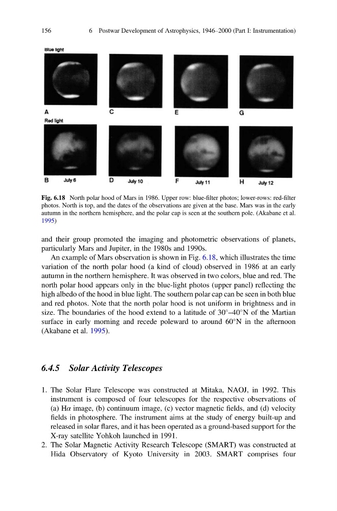
An example of Mars observation is shown in Fig. 6.18, which illustrates the time
variation of the north polar hood (a kind of cloud) observed in 1986 at an early
autumn in the northern hemisphere. It was observed in two colors, blue and red. The
north polar hood appears only in the blue-light photos (upper panel) reflecting the
high albedo of the hood in blue light. The southern polar cap can be seen in both blue
and red photos. Note that the north polar hood is not uniform in brightness and in
size. The boundaries of the hood extend to a latitude of 30
–40
N of the Martian
surface in early morning and recede poleward to around 60
N in the afternoon
(Akabane et al. 1995).
6.4.5 Solar Activity Telescopes
1. The Solar Flare Telescope was constructed at Mitaka, NAOJ, in 1992. This
instrument is composed of four telescopes for the respective observations of
(a) Hα image, (b) continuum image, (c) vector magnetic fields, and (d) velocity
fields in photosphere. The instrument aims at the study of energy built-up and
released in solar flares, and it has been operated as a ground-based support for the
X-ray satellite Yohkoh launched in 1991.
2. The Solar Magnetic Activity Research Telescope (SMART) was constructed at
Hida Observatory of Kyoto University in 2003. SMART comprises four
Fig. 6.18 North polar hood of Mars in 1986. Upper row: blue-filter photos; lower-rows: red-filter
photos. North is top, and the dates of the observations are given at the base. Mars was in the early
autumn in the northern hemisphere, and the polar cap is seen at the southern pole. (Akabane et al.
1995)
156
6 Postwar Development of Astrophysics, 1946–2000 (Part I: Instrumentation)
particularly Mars and Jupiter, in the 1980s and 1990s.
An example of Mars observation is shown in Fig. 6.18, which illustrates the time
variation of the north polar hood (a kind of cloud) observed in 1986 at an early
autumn in the northern hemisphere. It was observed in two colors, blue and red. The
north polar hood appears only in the blue-light photos (upper panel) reflecting the
high albedo of the hood in blue light. The southern polar cap can be seen in both blue
and red photos. Note that the north polar hood is not uniform in brightness and in
size. The boundaries of the hood extend to a latitude of 30
–40
N of the Martian
surface in early morning and recede poleward to around 60
N in the afternoon
(Akabane et al. 1995).
6.4.5 Solar Activity Telescopes
1. The Solar Flare Telescope was constructed at Mitaka, NAOJ, in 1992. This
instrument is composed of four telescopes for the respective observations of
(a) Hα image, (b) continuum image, (c) vector magnetic fields, and (d) velocity
fields in photosphere. The instrument aims at the study of energy built-up and
released in solar flares, and it has been operated as a ground-based support for the
X-ray satellite Yohkoh launched in 1991.
2. The Solar Magnetic Activity Research Telescope (SMART) was constructed at
Hida Observatory of Kyoto University in 2003. SMART comprises four
Fig. 6.18 North polar hood of Mars in 1986. Upper row: blue-filter photos; lower-rows: red-filter
photos. North is top, and the dates of the observations are given at the base. Mars was in the early
autumn in the northern hemisphere, and the polar cap is seen at the southern pole. (Akabane et al.
1995)
156
6 Postwar Development of Astrophysics, 1946–2000 (Part I: Instrumentation)