

5.4 Comparison with MC Calculations
49
10
1
10
2
10
3
10
4
(rad/sec)
0
0.5
1
1.5
2
2.5
3
S
B
z
( ) (T
2
/Hz)
10
-19
1
1.1
1.2
1.3
1.4
1.5
1.6
1.7
1.8
1.9
2
2.25
2.5
2.75
3
3.5
4
Temperature (K)
10
2
10
3
10
4
(rad/sec)
0
0.2
0.4
0.6
0.8
1
S ( ) (
0
2
/Hz)
10
-4
0
1
2
S
B
z
( ) (T
2
/Hz)
10
-22
1.2
1.23
1.26
1.29
1.32
1.35
1.4
1.45
1.5
1.55
1.6
1.7
1.8
2
2.25
2.5
3
3.5
4
1.6
Temperature (K)
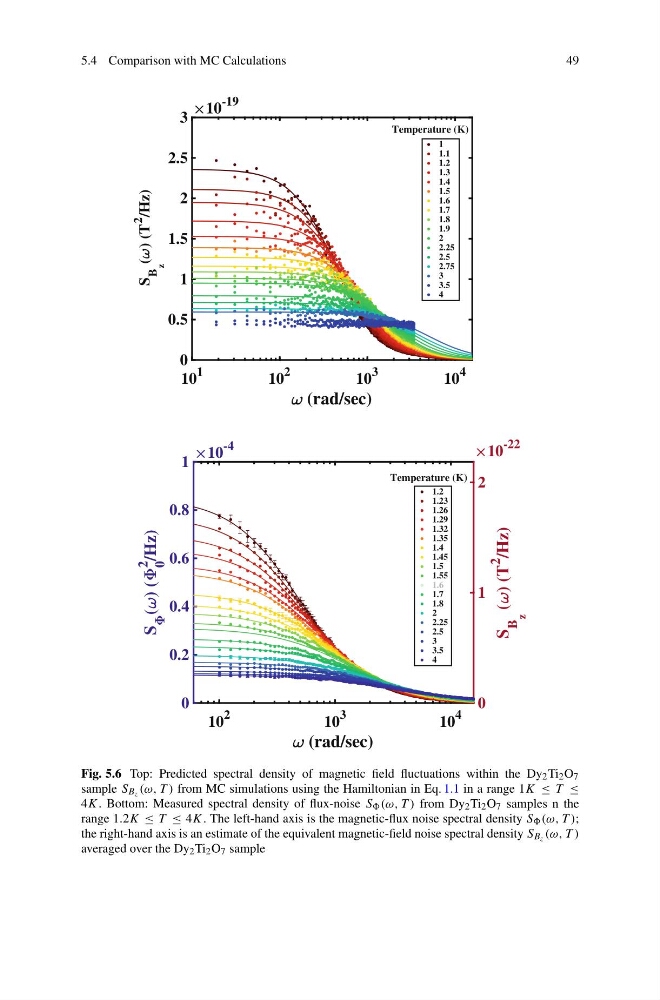
Fig. 5.6 Top: Predicted spectral density of magnetic field fluctuations within the Dy 2 Ti 2 O 7
sample S Bz (ω, T ) from MC simulations using the Hamiltonian in Eq. 1.1 in a range 1K ≤ T ≤
4K. Bottom: Measured spectral density of flux-noise S (ω, T ) from Dy 2 Ti 2 O 7 samples n the
range 1.2K ≤ T ≤ 4K. The left-hand axis is the magnetic-flux noise spectral density S (ω, T );
the right-hand axis is an estimate of the equivalent magnetic-field noise spectral density S Bz (ω, T )
averaged over the Dy 2 Ti 2 O 7 sample
49
10
1
10
2
10
3
10
4
(rad/sec)
0
0.5
1
1.5
2
2.5
3
S
B
z
( ) (T
2
/Hz)
10
-19
1
1.1
1.2
1.3
1.4
1.5
1.6
1.7
1.8
1.9
2
2.25
2.5
2.75
3
3.5
4
Temperature (K)
10
2
10
3
10
4
(rad/sec)
0
0.2
0.4
0.6
0.8
1
S ( ) (
0
2
/Hz)
10
-4
0
1
2
S
B
z
( ) (T
2
/Hz)
10
-22
1.2
1.23
1.26
1.29
1.32
1.35
1.4
1.45
1.5
1.55
1.6
1.7
1.8
2
2.25
2.5
3
3.5
4
1.6
Temperature (K)
Fig. 5.6 Top: Predicted spectral density of magnetic field fluctuations within the Dy 2 Ti 2 O 7
sample S Bz (ω, T ) from MC simulations using the Hamiltonian in Eq. 1.1 in a range 1K ≤ T ≤
4K. Bottom: Measured spectral density of flux-noise S (ω, T ) from Dy 2 Ti 2 O 7 samples n the
range 1.2K ≤ T ≤ 4K. The left-hand axis is the magnetic-flux noise spectral density S (ω, T );
the right-hand axis is an estimate of the equivalent magnetic-field noise spectral density S Bz (ω, T )
averaged over the Dy 2 Ti 2 O 7 sample